

We can use the MATCH function to get the last row in text data when working with excel spreadsheets. This can be done either with or without empty cells as thoroughly explained in this post.
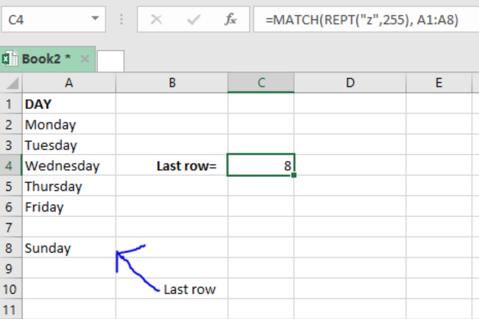 Figure 1: Using MATCH function to find last relative position of text data
Syntax of the formula
=MATCH(REPT(text, number_times), lookup_array)
Understanding the formula
For this formula to locate the last text in a rage, it uses the MATCH function in an approximate mode. There are two ways I which the approximate match mode can be enabled as shown below;
- Set the 3rd argument in MATCH to 1
- Omit the 3rd argument, thus setting the default to 1.
In the formula, we have the text, also referred to as the bigtext or big text, which is supposed to be a value that is bigger than any other value that will appear in the range. If it is numbers, then this will be the biggest number in the data provided. If it is alphabetical text, then this will be the text that appears at the most bottom if the text alphabetically sorted.
How the formula works
- MATCH function allows only 255 characters to appear in any lookup value. This is why we use the REPT function, to repeat “z” 255 times.
- In the event the MATCH function does not find this letter, then it will step back to the last text and return the position of that value.
Example
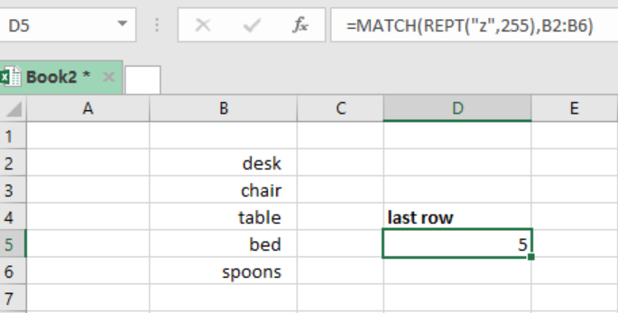 Figure 2: Using MATCH function to get the last relative position of a text data
Instant Connection to an Expert through our Excelchat Service
Most of the time, the problem you will need to solve will be more complex than a simple application of a formula or function. If you want to save hours of research and frustration, try our live Excelchat service! Our Excel Experts are available 24/7 to answer any Excel question you may have. We guarantee a connection within 30 seconds and a customized solution within 20 minutes.


Leave a Comment