

With the help of the MAX and MATCH functions in excel, we can now easily get the position of the maximum value in excel. This post provides a clear guide on how to use these functions to get the position of the max value in list.
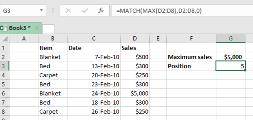 Figure 1: Finding position of max value in list
General syntax of the formula
=MATCH(MAX(range),range,0)
Where;
Range- refers to the range of values from which you want to find the position of the maximum value.
Understanding the formula
The combination of the MATCH and MAX functions in excel is very fundamental when it comes to getting the position of the maximum value.
How the formula works
- The formula is composed of two functions, the MATCH and MAX functions.
- Each of these functions play a fundamental role in making it possible for us to get the position of the max value.
- In the formula, the MAX function first extracts the maximum value from the supplied range. In the above case. The maximum value in the range is $5000
- The MAX function then supplies the max value to the MATCH function as a lookup value.
- Note that the lookup array is actually same as the range.
- We are also supposed to set the match_type to exact with the 0
- The MATCH function will then locate the maximum value in the range and return its relative position.
- The position can be that of a row number or a column number depending on the situations
Example
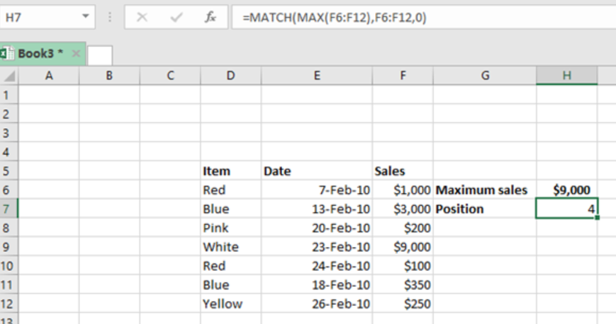 Figure 2: Example of how to find the relative position of max value in list
In this example, we want to find the relative position of the maximum value in the range F6:F12
To do this, we proceed as follows;
Step 1: Set up the data in the table as shown above
Step 2: Indicate where you want the result to appear
Step 3: In cell H7, put the formula =MATCH(MAX(F6:F12),F6:F12,0)
Step 4: Press enter to get the relative position of the maximum value.
Instant Connection to an Expert through our Excelchat Service
Most of the time, the problem you will need to solve will be more complex than a simple application of a formula or function. If you want to save hours of research and frustration, try our live Excelchat service! Our Excel Experts are available 24/7 to answer any Excel question you may have. We guarantee a connection within 30 seconds and a customized solution within 20 minutes.


Leave a Comment