

VLOOKUP is used to retrieve data from a data set using a lookup value or a criteria for a match. Sometimes, it is possible to only have a part of a criteria to use as a lookup value which requires a partial match.
Find a partial match in Excel with VLOOKUP
In performing a partial match with VLOOKUP, we make use of the wildcard character asterisk “*”. This tutorial will walk through the process of finding partial matches using wildcards.
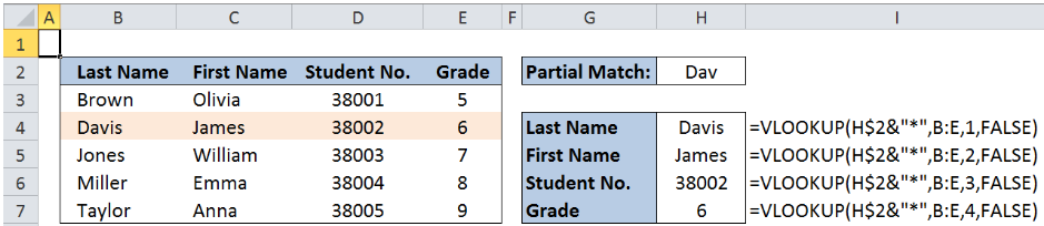 Figure 1. Final result for partial match with VLOOKUP
Formula using VLOOKUP
Working formula: =VLOOKUP(H$2&"*",B:E,1,FALSE)
Vlookup is used when we want to retrieve data from a given data set, by using the first column as the match criteria.
Syntax for partial match
=VLOOKUP(lookup_value, table_array, col_index_num, [range_lookup])
Where
- Lookup_value : the value we want to search
- Table_array: the range of cells containing the data we want to retrieve
- Col_index_num: the column number in the table_array corresponding to the information we want to retrieve, relative to the first column
- [range_lookup]: optional; value is either TRUE or FALSE;
- if TRUE or omitted, VLOOKUP returns either an exact or approximate match; it is important to sort the first column of the table_array in ascending order to ensure that VLOOKUP returns the correct value
- if FALSE, VLOOKUP will only find an exact match.
- Important note: When performing a partial match, range_lookup should always be FALSE for the wildcard match to work properly
Setting up the Data
Here we have a list of students with corresponding last names, first names, student numbers, and grade level. We want to find the details for the last name starting with “Dav”.
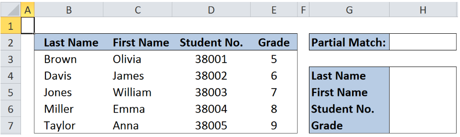 Figure 2. Sample data for partial match with VLOOKUP
Partial Match with VLOOKUP
We want to find the complete details for the last name starting with “Dav”.
In cell H2, enter the partial match criteria “Dav”.
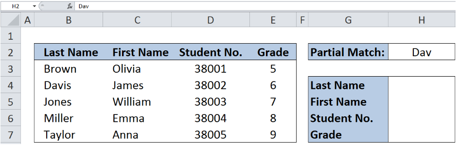 Figure 3. Entering the lookup value or partial match criteria : Dav
In cell H4, enter the formula:
=VLOOKUP(H$2&"*",B:E,1,FALSE)
Where:
- H$2&”*” is the criteria for the partial match, which translates to “Dav*”
- The asterisk “*” after Dav means any number of characters that may follow the word Dav
- Dav* means that we are looking for any value that starts with Dav, with zero or more characters afterward (example: Davis, Davidson, Davos)
- The dollar sign $ before 2 in H$2 ensures that when we copy the formula later, the row number for the criteria remains constant at row 2
- The ampersand & is used to concatenate or link the value for H2 and the asterisk “*”
- B:E is the table array or the range of data where we want to search for the last name starting with Dav; It is important to note that the first column for the array should be the column containing the partial match criteria
- 1 as the col_num_index means that we want to retrieve the data in column B that matches the criteria Dav*; col_num_index is determined relative to the first column;
- FALSE as the range_lookup means that we want VLOOKUP to return an exact match of the lookup_value or criteria
The formula returns Davis, which is the value in column B that matches the lookup value Dav*.
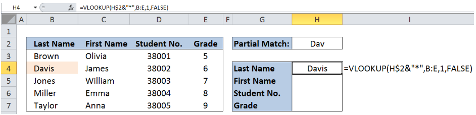 Figure 4. Entering the VLOOKUP formula for last name
Retrieving the First Name for Davis
Now we want to retrieve the corresponding first name for Davis.
In cell H5, enter the formula:
=VLOOKUP(H$2&"*",B:E,2,FALSE)
Note that the formula is similar to the above example.
The lookup_value is still Dav*, which matches Davis in column B. However, the col_num_index is now “2”. This means that we want to retrieve the corresponding value in column C, which is the 2nd column relative to column B.
The formula returns the value “James”.
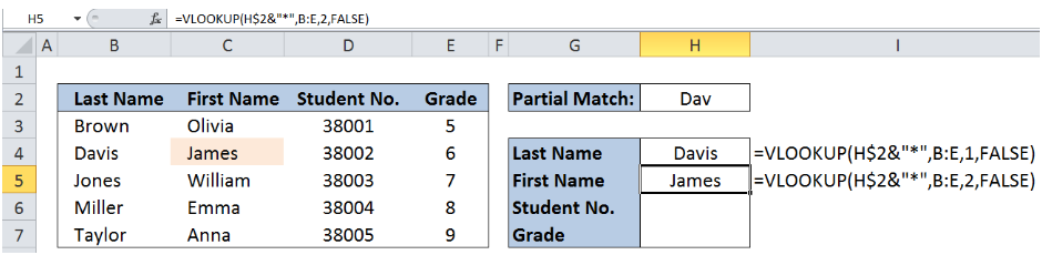 Figure 5. Entering the VLOOKUP formula for first name
To complete the other details, enter the formula in cells H6 and H7 as shown below:
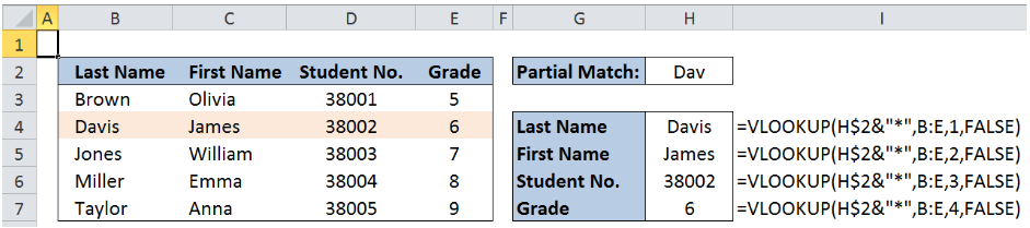 Figure 6. Output: Partial match with VLOOKUP for “Dav”
Another example
Suppose we want to retrieve the details for the last name starting with “Mil”.
Below table summarizes the formula and VLOOKUP results.
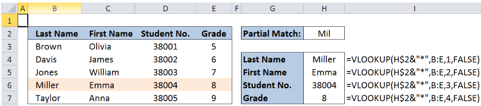 Figure 7. Output: Partial match with VLOOKUP for “Mil”
Most of the time, the problem you will need to solve will be more complex than a simple application of a formula or function. If you want to save hours of research and frustration, try our live Excelchat service! Our Excel Experts are available 24/7 to answer any Excel question you may have. We guarantee a connection within 30 seconds and a customized solution within 20 minutes.


Leave a Comment