Here is How to Use Excel’s MATCH Function

We can use excel MATCH FUNCTION to locate the position of a lookup value in a column, row, or table. Approximate and exact matching are supported by MATCH FUNCTION and wildcards (* ?) for partial matches. The steps below will walk through the process.

Figure 1- How to Use Excel MATCH Function

Syntax

=MATCH(lookup_value,lookup_array,match_type)

• lookup_value: This is the value to match in lookup_array.
• lookup_array – This is a range of cells or an array reference.
• match_type [optional]: How to match, specified as -1, 0, or 1. Default is 1.

Formulas

Exact match: =MATCH(C4,$B$4:$B$8,0)

Approximate match: =MATCH(H3,F4:F8,1)

Wildcard match: =MATCH(L3,J4:J8,0)

Setting up the Data

We will use the data in figure 2 to find an exact match for the names Jude, Sam, and Paul. We will also find the lookup result for 400 and er*.

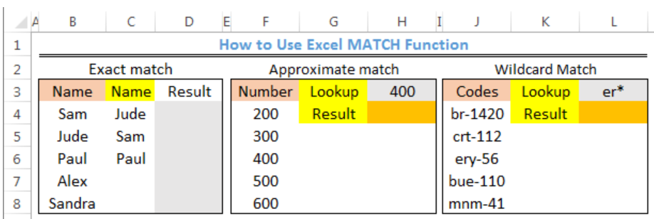Figure 2 – Setting up the Data

Exact MATCH

If match_type is 0, the MATCH FUNCTION will return the first value that is exactly equal to the lookup_value.

• We will click on Cell D4
• We will insert the formula below into Cell D4
  =MATCH(C4,$B$4:$B$8,0)
• We will press the enter key

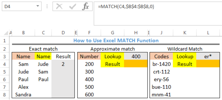Figure 3- Exact Match Result for Jude

• We will click on Cell D4 again
• We will double click on the fill handle tool which is the small plus sign you see at the bottom right of Cell D4. Select and drag down to copy the formula to Cell D6.

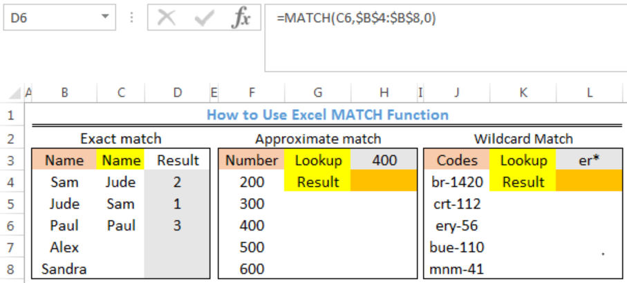Figure 4- Results for Exact Match

Approximate MATCH

If match_type is 1, the MATCH function will find the largest value that is less than or equal to the lookup_value. Here, the lookup_array must be sorted in ascending order.

• We will click on Cell H4
• We will insert the formula below into Cell H4
  =MATCH(H3,F4:F8,1)
• We will press the enter key

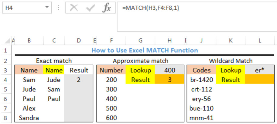Figure 5- Result for Approximate Match

Wildcard Match

If match_type is 0, the MATCH function can find a match with wildcards. Here, the MATCH FUNCTION will find the code that begins with “er”

• We will click on Cell L4
• We will insert the formula below into Cell L4
  =MATCH(L3,J4:J8,0)
• We will press the enter key

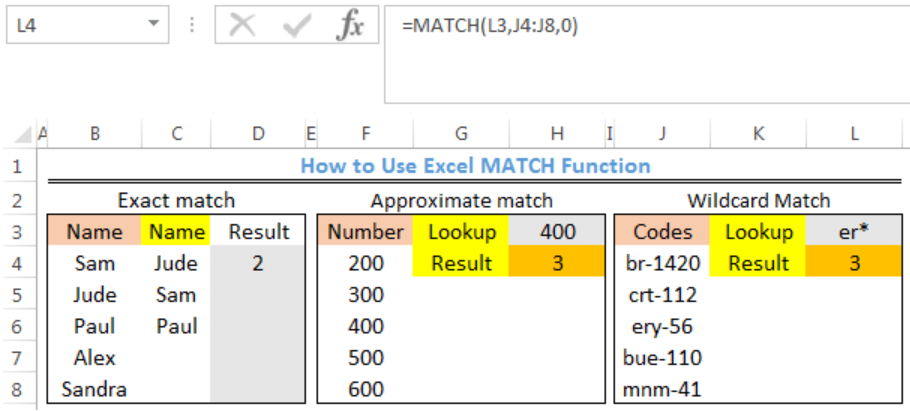Figure 6- Result for Wildcard Match

Note

• If match_type is -1, the MATCH FUNCTION will find the smallest value that is greater than or equal to the lookup_value. The lookup_array must be sorted in descending order
• If we omit match_type, it is assumed to be 1
• MATCH FUNCTION is not case-sensitive.
• The MATCH FUNCTION returns #N/A error if no match is found
• If the match_type is 0 and lookup_value is text, then, wildcard characters like question mark (?) and asterisk (*) can be used in lookup_value

Instant Connection to an Expert through our Excelchat Service

Most of the time, the problem you will need to solve will be more complex than a simple application of a formula or function. If you want to save hours of research and frustration, try our live Excelchat service! Our Excel Experts are available 24/7 to answer any Excel question you may have. We guarantee a connection within 30 seconds and a customized solution within 20 minutes.