

Excel allows a user to lookup values across multiple sheets using the VLOOKUP function. This step by step tutorial will assist all levels of Excel users to lookup values across multiple sheets in Excel
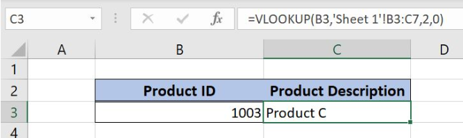 Figure 1. The result of the VLOOKUP function
Syntax of the VLOOKUP Formula
The generic formula for the VLOOKUP function is:
=VLOOKUP(lookup_value, table_array, col_index_num, range_lookup)
The parameters of the VLOOKUP function are:
- lookup_value – a value that we want to find in a table_array
- table_array – a range in which we want to lookup
- col_index_num – a column number in table_array from which we would like to get a value
- range_lookup – default value 0. This means that we want to find an exact match for a lookup value.
Setting up Our Data for the VLOOKUP Function
Let’s look at the structure of the data that we will use. In the range B2:C7 of Sheet 1, we have a table from which we want to pull data, while in the cell F3 of Sheet 2 we want to get a value. Tables consist of the columns “Product ID” and “Product Description”.
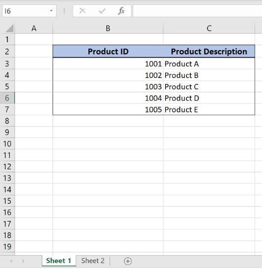 Figure 2. The data table in Sheet 1 that we will use in the VLOOKUP example
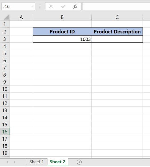 Figure 3. Sheet 2 where we want to get a result
Get the Product Description from Another Sheet Using the VLOOKUP Function
Our goal is to obtain the “Product Description” from the Sheet 1 and populate it in Sheet 2, into the cell C3.
The formula looks like:
=VLOOKUP(B3, 'Sheet 1'!B3:C7, 2, 0)
In our example, the lookup_value is the B3 cell in “Product ID” column of Sheet 2. The parameter table_array is ‘Sheet 1’!B3:C7 of Sheet 1 because we want to find value from the range B3:B7. When we reference the sheet we have to put the name of the Worksheet under single quotations and exclamation mark. Col_index_num has value 2, as we want to pull value from the second column of the range. Finally, range_lookup has value 0, because we want to find an exact match of “Product ID” values.
To apply the VLOOKUP function, we need to follow these steps:
- Select cell C3 and click on it
- Insert the formula:
=VLOOKUP(B3, 'Sheet 1'!B3:C7, 2, 0) - Press enter.
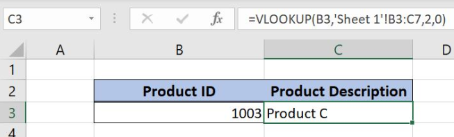 Figure 4. Using the VLOOKUP function
As a result, we will get Product C in the cell C3 of Sheet 2. As you can see, the value of “Product Description” in C3 in Sheet 1 table is Product C. The function pulls this value and returns it to the cell C3 as a result.
Most of the time, the problem you will need to solve will be more complex than a simple application of a formula or function. If you want to save hours of research and frustration, try our live Excelchat service! Our Excel Experts are available 24/7 to answer any Excel question you may have. We guarantee a connection within 30 seconds and a customized solution within 20 minutes.


Leave a Comment