

Excel has some very efficient ways to find the max value in a list or range. We can also find the corresponding values of the greatest value easily. We can combine the INDEX, MATCH and MAX functions to extract the corresponding values. In this tutorial, we will learn how to get information corresponding to max value in Excel.
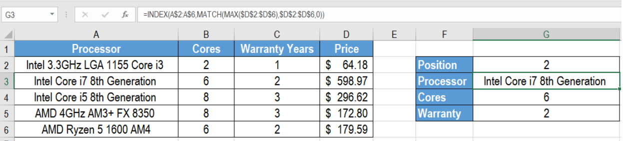 Figure 1. Example of Getting Information Corresponding to Max Value
Generic Formula
=INDEX(Range1,MATCH(MAX(Range2),Range2,0)
How the Formula Works
Firstly, the function MAX gets the max value from Range2. We provide this value to the MATCH function as the first argument which is the lookup_value. Here, The lookup_array is also Range2. The match_type is set to 0 which represents an exact match.
The MATCH function returns the relative position of the maximum value in Range2. We supply this value to the INDEX function as the second argument. This is the row_number. The range is Range1, which is the lookup_array. Thus, the INDEX function returns the value in the relative position in Range1. This is based on the max value in Range2.
Setting Up Data
The following example uses a microprocessor information data set. The processor names are in column A. Column B, C and D contains the price, cores and warranty years.
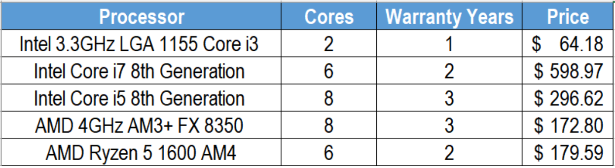 Figure 2. The Sample Data Set
To get the corresponding information to the max value:
- We need to select cell G3.
- Assign the formula
=INDEX(A$2:A$6,MATCH(MAX($D$2:$D$6),$D$2:$D$6,0))to cell G3. - Press Enter.
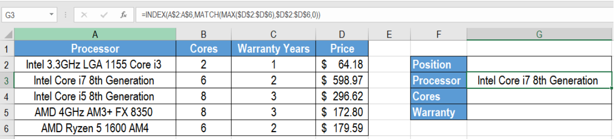 Figure 3. Assigning the Formula to Get the Corresponding Values to the Max Value
- Drag the formula using the fill handle in the bottom right to copy the formula to the cells below. We have to change the lookup_array reference to the respective columns to get the appropriate result.
- To get the position in cell G2, we need to assign the formula
=MATCH(MAX($D$2:$D$6),$D$2:$D$6,0)to cell G2.
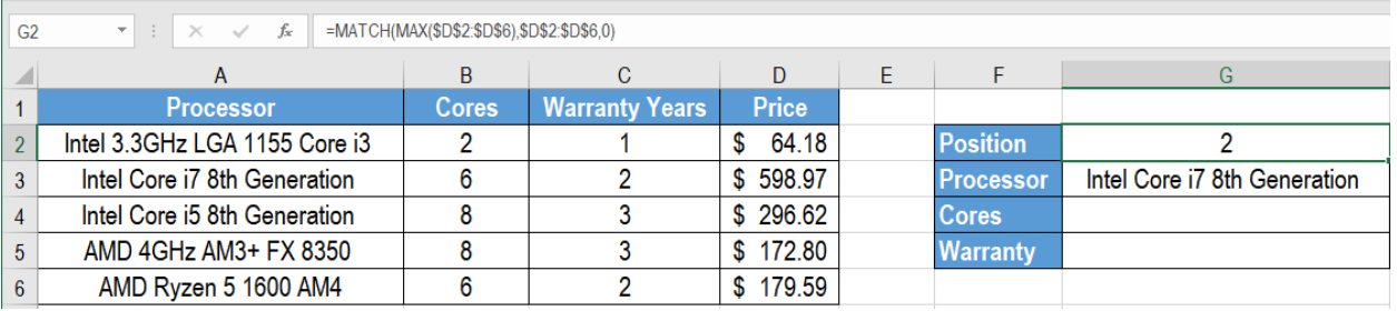 Figure 4. Getting the Position of the Max Value
This will find the max value which is $598.97 and display the corresponding information in column G.
Notes
- If there are duplicate values, this formula returns the first match.
- If the values in Range2 are not valid numbers, this formula returns an #VALUE error.
Most of the time, the problem you will need to solve will be more complex than a simple application of a formula or function. If you want to save hours of research and frustration, try our live Excelchat service! Our Excel Experts are available 24/7 to answer any Excel question you may have. We guarantee a connection within 30 seconds and a customized solution within 20 minutes.


Leave a Comment