Break ties with helper column and COUNTIF

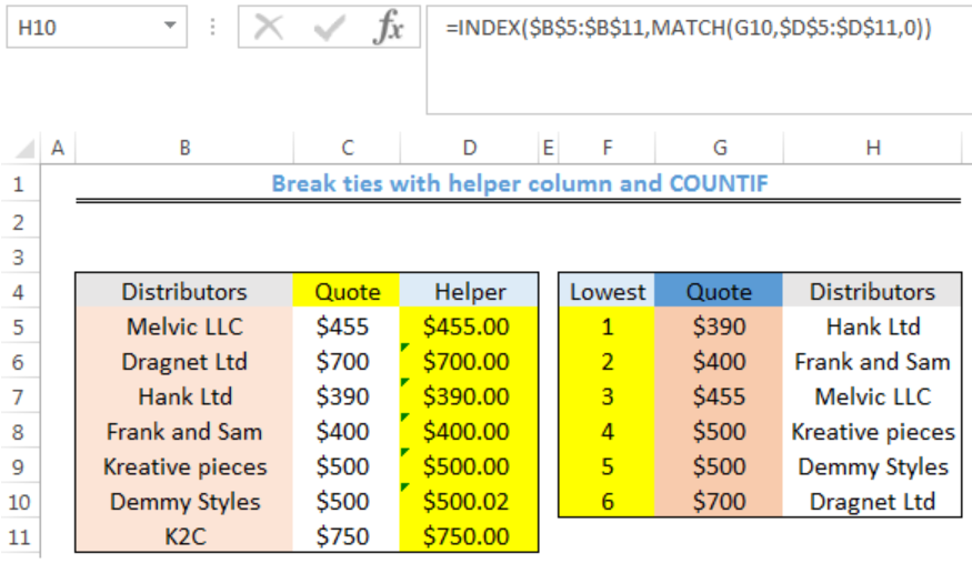
We can break ties (the same values) in a data with the COUNTIF function and a helper column. This effectively removes duplicates and removes confusion about the data. The steps below will guide all levels of excel users through the process.

Figure 1: How to Break ties with helper column and COUNTIF

General Formula

=A1+(COUNTIF(exp_rng,A1)-1)*adjustment

Formulas

Helper Column: =C5+(COUNTIF($C$5:C5,C5)-1)*0.02

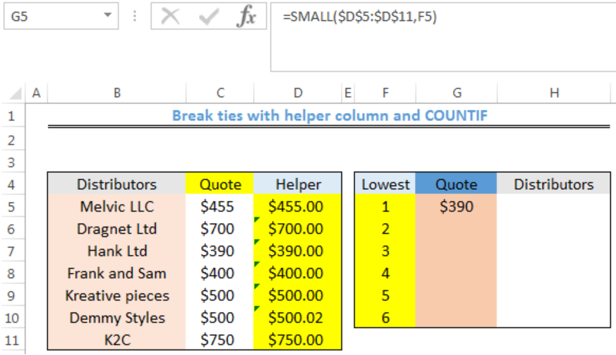
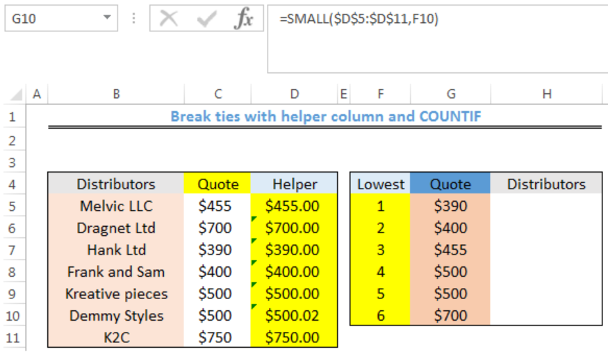
Quote: =SMALL($D$5:$D$11,F5)

Distributors: =INDEX($B$5:$B$11,MATCH(G5,$D$5:$D$11,0))

Setting up the Data

• We will set up the data by inputting the Distributors and their Quotes in Column B and Column C respectively
• After generating the values for the helper column, we will rank the quotes of the distributors to get the 6 lowest quotes.

Figure 2: Setting up the Data

Generating the Helper Column

• We will click on Cell D5
• We will insert the formula below into the cell
  =C5+(COUNTIF($C$5:C5,C5)-1)*0.02
• We will press the enter key

Figure 3: Generating the Helper Column

• We will click on Cell D5 again
• We will double click on the fill handle tool which is the small plus sign you see at the bottom right of Cell D5. Select and drag down to copy the formula to other cells.

Figure 4: Helper Column Generated

• We will notice that the quotes of Kreative pieces and Demmy Styles have been distinguished with the helper column

Getting the Quotes

• We will click on Cell G5
• We will insert the formula below into the cell
  =SMALL($D$5:$D$11,F5)
• We will press the enter key

Figure 5: Getting the Quotes

• We will click on Cell G5 again
• We will double click on the fill handle tool which is the small plus sign you see at the bottom right of Cell G5. Select and drag down to copy the formula to other cells.

Figure 6: Generated Quotes

Getting the Distributors

• We will click on Cell H5
• We will insert the formula below into the cell
  =INDEX($B$5:$B$11,MATCH(G5,$D$5:$D$11,0))
• We will press the enter key

Figure 7: Getting the Distributors

• We will click on Cell H5 again
• We will double click on the fill handle tool which is the small plus sign you see at the bottom right of Cell H5. Select and drag down to copy the formula to other cells.

Figure 8: Distributors

Explanation

=C5+(COUNTIF($C$5:C5,C5)-1)*0.02

If we had ranked the quote with the SMALL FUNCTION without the helper column, we will have two ranks with $500 and we won’t know the distributors the quotes belong to. The helper column sorts this out by leaving the first tie value as it is and uses the multiplier (0.02) from the formula to rank the second tie value.

COUNTIF function utilizes an expanding range to return a running count of occurrences, rather than a total count for each value.

=COUNTIF($C$5:C5,C5)

1 is subtracted from the result and all non-duplicate values will be zero. The result is multiplied by 0.02. This value is the “adjustment.” The adjustment should be kept small so that we do not impact the original value.

Instant Connection to an Expert through our Excelchat Service

Most of the time, the problem you will need to solve will be more complex than a simple application of a formula or function. If you want to save hours of research and frustration, try our live Excelchat service! Our Excel Experts are available 24/7 to answer any Excel question you may have. We guarantee a connection within 30 seconds and a customized solution within 20 minutes.