

While using the VLOOKUP function in Excel, sometimes we need to lookup multiple tables. In order to create the dynamic VLOOKUP formula, we will nest the INDIRECT function inside of a VLOOKUP function to dynamically reference multiple tables within the lookup formula. In this tutorial, we will see how to create a dynamic lookup table with INDIRECT function.
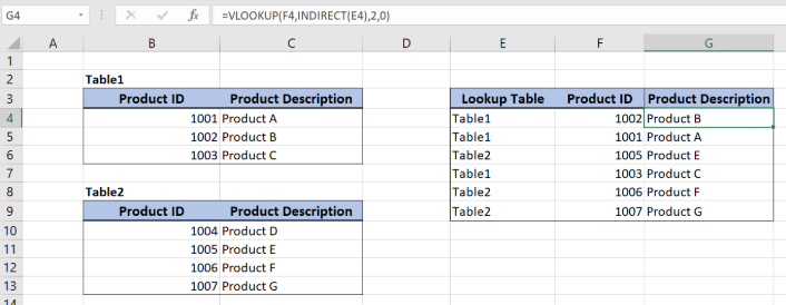 Figure 1. Final result
Syntax of the INDIRECT and VLOOKUP formula
The generic formula for creating a dynamic lookup table:
=VLOOKUP(lookup_value, INDIRECT(text), 2, 0)
The components of the formula are:
- INDIRECT – by this Excel function we can reference the specific sheet and the cell range where we want to summarize the data
- VLOOKUP –
=VLOOKUP(lookup_value, table_array, col_index_num, range_lookup)
The parameters of the VLOOKUP function are:
- lookup_value – a value that we want to find in the VLOOKUP table
- table_array – a range in which we want to lookup
- col_index_num – a column number from which we would like to pull a value
- range_lookup – default value 0. This means that we want to find an exact match for a lookup value.
- Named range – a range of values which we want to sum
Setting up Our Data
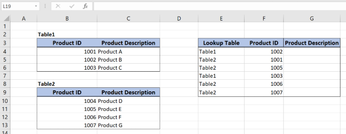 Figure 2. Data structure for a dynamic VLOOKUP function
In the ranges B3:C6 and B9:C13, we have two tables with similar structures, but different data values. The tables consist of “Product ID” (column B) and “Product Description” (column C). In the column G, we want to get Product description from the two VLOOKUP tables, based on “Lookup table” and “Product ID” cells values (columns E and F).
To be able to reference dynamically the table, we will first need to create named ranges for both VLOOKUP tables.
Create Named Ranges
Follow these steps to create named ranges:
- Select the table for which we want to create a named range (B3:C6)
- In Formula tab click on the Name Manager
- In popup screen select New
- A new window will appear and we will have to define “Name”, “Scope” and “Refers to”
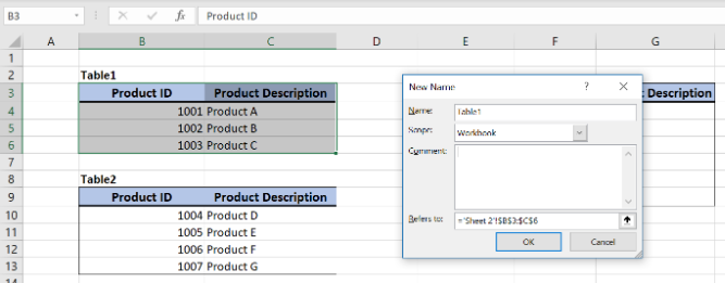 Figure 3. How to create named range in Name Manager
- Name of the range will be “Table1”, Scope will be the Workbook, while Refers to will be Table1 (B3:C6)
- Just click OK and we created a named range “Table1”
- In order to create the same named range for the other table, just repeat steps above, but first select the range B9:C13.
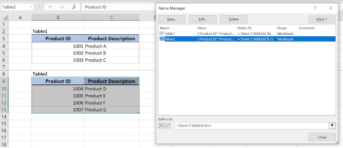 Figure 4. Named ranges for Product tables
- As a result, in Figure 3, we created two named ranges referencing to Product data
Application of the modified VLOOKUP formula with the INDIRECT function
Our goal is to get Product description in the column G, based on Product ID from the column F. Using the INDIRECT function, we will decide which table to use in VLOOKUP (column E).
The formula looks like:
=VLOOKUP(F4, INDIRECT(E4), 2, 0)
In our example, the lookup_value is the cell F4. The parameter table_array. The parameter table_array is the result of INDIRECT(E4) function. Col_index_numhas value 2, as we want to pull value from the second column of the range. Finally, range_lookup has value 0, because we want to find an exact match of “Lookup column” values.
To apply the VLOOKUP with dynamic tables, we need to follow these steps:
- Define named ranges for the tables
- Select cell G4 and click on it
- Insert the formula:
=VLOOKUP(F4, INDIRECT(E4), 2, 0) - Press enter
Figure 5. Dynamic Lookup table with INDIRECT function
The INDIRECT(E4) function returns “Table1”, which will be table_array parameter in the VLOOKUP function. This means that we want to find Product B (F4) in Table1 (B3:C6). The value of the Product description for 1002 in Table1 is Product B, which is the result of the function in the cell G4.
Most of the time, the problem we will need to solve will be more complex than a simple application of a formula or function. If you want to save hours of research and frustration, try our live Excelchat service! Our Excel Experts are available 24/7 to answer any Excel question you may have. We guarantee a connection within 30 seconds and a customized solution within 20 minutes.


Leave a Comment