

When we want to get the exact position of a given value in a column, row or table, we can use the Excel MATCH function. To fully understand how the function works, please read this post to the end.
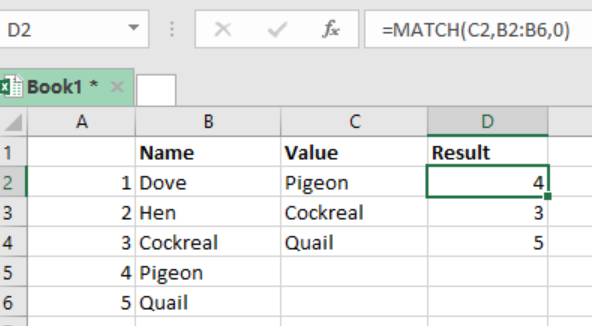 Figure 1: Using Excel MATCH function to find relative positions
General syntax of the formula
=MATCH (look_up, look_array, [match_type])
Where;
- Lookup_value– value to match in look_up array
- Lookup_array– refers to the range of cells or array reference
- Match_type– shows how you want to match. Default is 1
How the MATCH function works
We use the MATCH function when we want to find the relative position of an item in an array. This function is very flexible given that it has different matching modes.
When used together with INDEX, MATCH can also help to retrieve a value at the matched position.
Different match types in MATCH function
- Match_type 1: this shows that the MATCH function will find the largest value which is less or equal to the lookup_value. Here, you will have to sort the lookup_array in ascending order.
- Match_type 0: here, the MATCH function will find the first value that is exactly equal to the lookup_value. You don’t have to sort the lookup_array when zero is your preferred match_type.
- Match_type -1: the MATCH function will find the smallest value which is greater than or equal to the lookup_value. You will have to sort the lookup_array in a descending order.
Note
When the match_type is omitted, then it will be assumed to be 1.
Also, all these match_types will return the exact match of what you are seeking.
Example
In this example, we want to find the relative positions of Dennis and Juliet. To do this, proceed as follows:
Step 1: Prepare your data sheet, complete with the names, value column as well as Result column
Step 2: Click in the cell where you want to get the result
Step 3: Write the formula in the active cell, i.e. =MATCH (C2,A1:A5,0)
Step 4: Press Enter
Step 5: Do the same for the other items.
Most of the time, the problem you will need to solve will be more complex than a simple application of a formula or function. If you want to save hours of research and frustration, try our live Excelchat service! Our Excel Experts are available 24/7 to answer any Excel question you may have. We guarantee a connection within 30 seconds and a customized solution within 20 minutes.


Leave a Comment