

Excel allows a user to get an internal rate of return of an investment using the IRR function. This step by step tutorial will assist all levels of Excel users in getting an IRR of an investment.
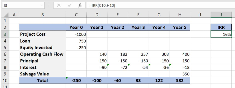 Figure 1. The result of the equity IRR function
Syntax of the SUM Formula
The generic formula for the SUM function is:
=SUM(number1, [number2], [number3],... )
The parameters of the SUM function are:
- number1, [number2], [number3],… – numbers that we want to summarize, or a range containing numbers.
Syntax of the IRR Formula
The generic formula for the IRR function is:
=IRR (values, [guess])
The parameters of the IRR function are:
- values – a range of cells containing values, including initial investment and incomes. The investment must have a negative sign, as it is a cost
- [guess] – an estimated value for the expected IRR. This parameter is non-mandatory. If it’s omitted, the function will take a default value of 0.1 (=10%).
Setting up Our Data for the Equity IRR Function
Let’s look at the structure of the data we will use. In columns C:H, we have years 0-5. In rows, we have incomes and costs per year. In cells C10:H10, we need to get the sum for each year. Finally, in the cell J3, we want to calculate the IRR for the specified cash-flow.
As we can see, Interest in row 8, is calculated based on loan and incomes, using the formula =-1*($C$4+SUM($C$7:C7))*.12
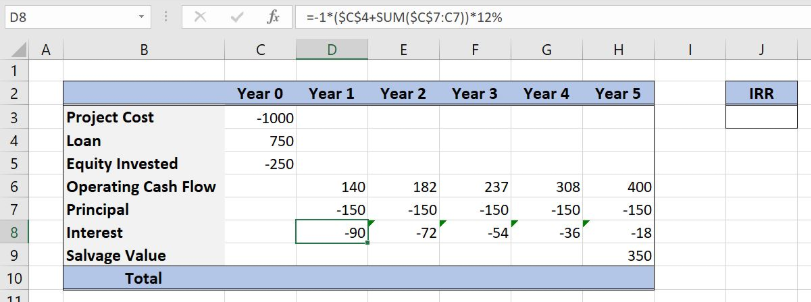 Figure 2. Data that we will use in the equity IRR example
Get an IRR of Values Using the IRR Function
In our example, we first want to calculate the sum for all years.
The formula for summarizing looks like:
=SUM(C5:C9)
The parameter numbers of the function is the range C5:C9.
To apply the SUM function, we need to follow these steps:
- Select cell C10 and click on it
- Insert the formula:
=SUM(C5:C9) - Press enter
- Drag the formula right to the other cells in the row by clicking and dragging the little “+” icon at the bottom-right of the cell.
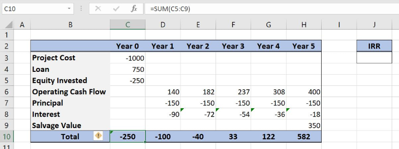 Figure 3. Using the SUM function to sum costs and incomes for every year
Finally, the result in the cell C10 is -250, which is the sum of costs and incomes for the Year 0. Now, we can calculate the IRR using the IRR function and sums for every year.
The formula for IRR looks like:
=IRR(C10:H10)
The parameter values of the function is the range C10:H10.
To apply the IRR function, we need to follow these steps:
- Select cell J3 and click on it
- Insert the formula:
=IRR(C10:H10) - Press enter.
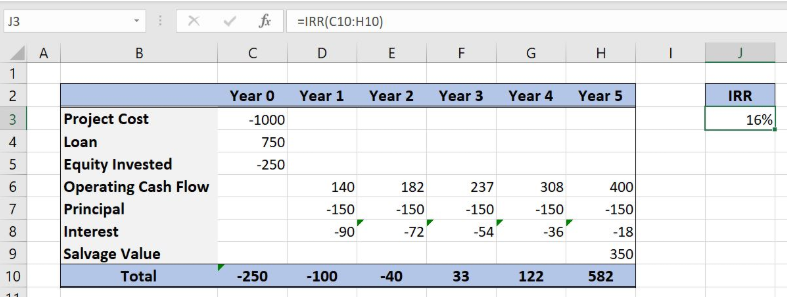 Figure 4. Using the IRR function to calculate the equity IRR
Finally, the internal rate of return in the cell J3 is 16%.
Most of the time, the problem you will need to solve will be more complex than a simple application of a formula or function. If you want to save hours of research and frustration, try our live Excelchat service! Our Excel Experts are available 24/7 to answer any Excel question you may have. We guarantee a connection within 30 seconds and a customized solution within 20 minutes.


Leave a Comment