

Excel allows a user to get an internal rate of return and a net present value of an investment using the NPV and IRR functions. This step by step tutorial will assist all levels of Excel users in calculating NPV and IRR Excel.
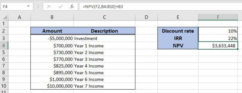 Figure 1. The result of the NPV and IRR functions
Syntax of the NPV Formula
The generic formula for the NPV function is:
=NPV(rate, values)
The parameter of the NPV function is:
- rate – a discount rate for the investment period
- values – values representing an investment (with a negative sign) and returns over periods.
Syntax of the IRR Formula
The generic formula for the IRR function is:
=IRR(values, [guess])
The parameter of the IRR function is:
- values – a range of cells containing values, including initial investment and incomes. The investment must have a negative sign, as it is a cost
- [guess] – an estimated value for the expected IRR. This parameter is non-mandatory. If it’s omitted, the function will take a default value of 0.1 (=10%).
Setting up Our Data for the NPV and IRR Functions
Let’s look at the structure of the data we will use. In column B (“Amount”), we have values including initial investment and yearly incomes. In column C (“Description”) we have a description of every amount. The discount rate is in F2. In the cell F3, we want to get the IRR, while in F4 NPV.
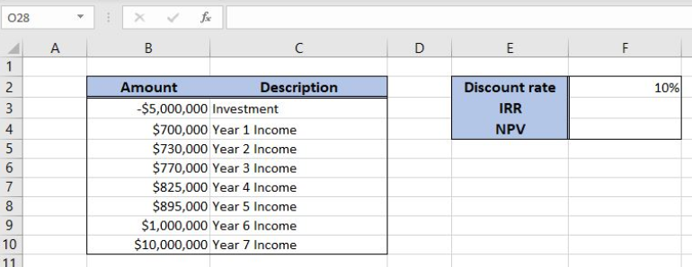 Figure 2. Data that we will use in the NPV and IRR example
Get an NPV of Values Using the NPV Function
In our example, we want to get the NPV of the values in the range B3:B10. The result will be in the cell F4.
The formula looks like:
=NPV(F2, B4:B10) + B3
The parameter rate is the cell F2, while the values are in the range B4:B10. We omit the first value from B3, as it is negative and add it to the function result.
To apply the NPV function, we need to follow these steps:
- Select cell E3 and click on it
- Insert the formula:
=NPV(F2, B4:B10) + B3 - Press enter.
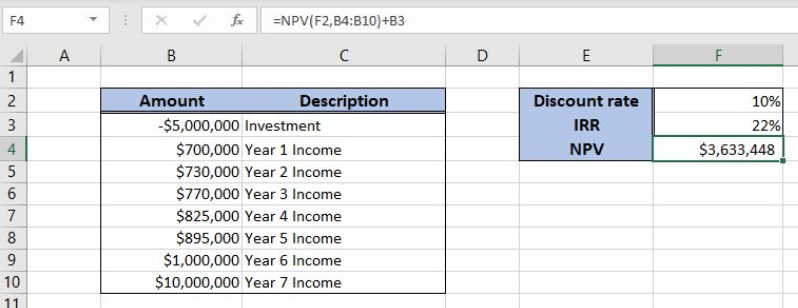 Figure 3. Using the NPV function to get the net present value of the investment
Finally, the result in the cell F4 is $3,633,448, which is the net present value of the investment and returns with the discount rate of 10%.
Get an IRR of Values Using the IRR Function
In this example, we want to get the IRR of the values in the range B3:B10. The result will be in the cell F3.
The formula looks like:
=IRR(B3:B10)
The parameter values is the range B3:B10
To apply the IRR function, we need to follow these steps:
- Select cell F3 and click on it
- Insert the formula:
=IRR(B3:B10) - Press enter.
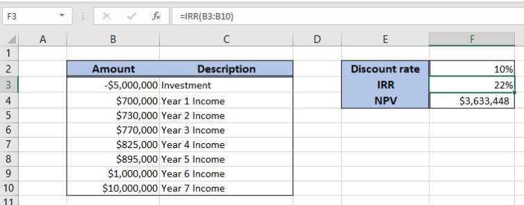 Figure 4. Using the IRR function to get the internal rate of the investment
Finally, the result in the cell E3 is 22%, which is the internal rate of the investment.
Most of the time, the problem you will need to solve will be more complex than a simple application of a formula or function. If you want to save hours of research and frustration, try our live Excelchat service! Our Excel Experts are available 24/7 to answer any Excel question you may have. We guarantee a connection within 30 seconds and a customized solution within 20 minutes.


Leave a Comment