How to Use the INDEX Function in Excel

The INDEX function returns a value or the reference to a value from within a table or range. It is used to fetch values from tabular data when you have the row and column numbers of the lookup value.

How to use Excel’s INDEX function

The INDEX function in Excel has two formats, the Array Format (which is the most basic format), and the Range Format. In this tutorial, you will learn how to use both formats of the INDEX function in Excel.

The Array Format

Syntax

The Array format of the Index function in Excel is used when you want to look up a reference to a cell within a single range. The syntax of the function is:

=INDEX (array, row_num, [col_num], [area_num])

Arguments

array – Required. It is a range of cells, or an array constant. If the array contains only one row or column, the corresponding row_num or col_num argument is optional. If it has more than one row and more than one column, and only row_num or col_num is used, INDEX returns an array of the entire row or column in the array.

row_num – Required. It is the position of the row from which the value is to be fetched. If omitted, col_num is required.

[col_num] – Optional. It is the column position in the reference or array. If omitted, row_num is required.

Returns

The value of an element in a table or an array, selected by the row and column number indexes.

Notes

• If both the row_num and col_num arguments are used, INDEX returns the value in the cell at the intersection of the two.
• If row_num and col_num are both set to 0 (zero), INDEX returns the array of values for the entire column or row, respectively. To use values returned as an array, enter the INDEX function as an array formula in a horizontal range of cells for a row, and in a vertical range of cells for a column. To enter an array formula, press CTRL+SHIFT+ENTER.

The Range Format

Syntax

The Range format of the Index function can be used to extract references from ranges that are made up of more than one area. The syntax of the function is:

INDEX( range, row_num, [col_num], [area_num] )

Arguments

Range – Required. The specified array or range of cells. If multiple areas are inserted directly into the function, the individual areas should be separated by commas and surrounded by brackets (ie.  A1:B2, C3:D4, etc).

row_num – Required. It is the row number of the specified area. If set to zero or blank, this defaults to all rows of the specified area within the supplied range.

[col_num] – Optional. Denotes the column number of the specified area. If set to zero or blank, this defaults to all columns of the specified area within the supplied range.

[area_num] – Optional. It is the range in reference that should be used. If this argument is omitted, it defaults to the value 1 (i.e., the reference is taken from the first area in the supplied range.

Returns

Extract references from ranges that are made up of more than one area.

Notes

• After Reference and Area_num have selected a particular range, row_num and col_num select a particular cell: row_num 1 is the first row in the range, col_num 1 is the first column, and so on. The reference returned by INDEX is the intersection of Row_num and Column_num.
• If you set row_num or column_num to 0 (zero), INDEX returns an array of the reference for the entire column or row, respectively. 
• row_num, column_num, and area_num must point to a cell within reference; otherwise, INDEX returns the #REF! error. If row_num and col_num are omitted, INDEX returns the area in reference specified by area_num.
• The result of the INDEX function is a reference and is interpreted as such by other formulas. Depending on the formula, the return value of INDEX may be used as a reference or as a value.

Examples

In the following examples, you will learn how to use the array format of the INDEX function.

Using the INDEX Function from the Dialog Box

To enter the INDEX function and arguments using the dialog box for the

example image:

1. Click on cell E2, which is the location where the result will be displayed.
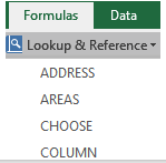
2. Click on the Formulas tab of the ribbon menu.
3. Choose Lookup and Reference from the ribbon to open the function drop-down list.
4. Click on INDEX in the list to bring up the function’s dialog box.
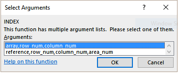
5. In the Select Arguments box, select the option that refers to the array array, row_num, col_num.
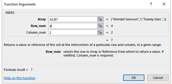
6. Highlight cells A2 to A8 in the worksheet to enter the array in the dialog box.
7. Click on the row_num line in the dialog box.
8. Insert the number 4 where Excel will fetch the value from.
9. Click on the col_num line in the dialog box.
10. Enter the number 2 on this line to return the value from column 2 which is Years of Experience.
11. Click OK to complete the function and close the dialog box.
    
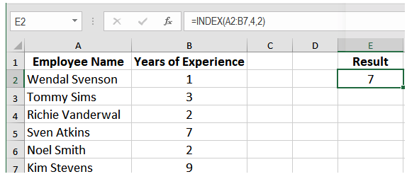
12. The number 7 appears in cell E2 since the employee in row four, Sven Atkins has 7 years of experience.

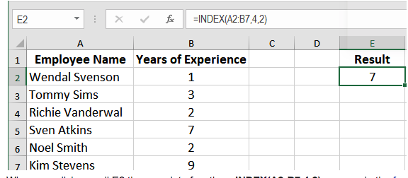
When you click on cell E2 the complete function =INDEX(A2:B7,4,2) appears in the formula bar above the worksheet.

Index Function Excel (Array Format)

In the following example, assign the formula =INDEX(A2:B7,4,2) to cell E2. The Index function returns a reference to row 4 of the range A2:B7, which is cell B5. This has the value 7.

Index Function Excel (Range Format)

In the following example, to find the Production hour of the month Jun, assign the formula =INDEX((C2:D5,D7:E10,F2:G5),3,2,2) to cell G8.

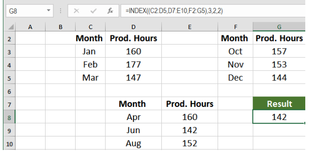
The Index function returns a reference to row 2 and column 2 of the 3rd area in the supplied range. This is cell G8, which evaluates to the value 142.

Still need some help with Excel formatting or have other questions about Excel? Connect with a live Excel expert here for some 1 on 1 help. Your first session is always free.