

VLOOKUP is one of the lookup and reference functions in Excel is used to find values in a specified range by “row”. It compares them row-wise until it finds a match. In order for VLOOKUP to work, the lookup value must be on the left-most column on the table array. If your lookup value is not on the first column of the array, you will see the #N/A error. In this tutorial, we will look at some workarounds when the value is not in the first column.
Using VLOOKUP for matches when the lookup value isn’t in the first column
We will use the employee records dataset for demonstration. Here we have the employee information on cells A2:C8. For each employee, we have their Employee ID, Name and departments. In the following table, we want to retrieve the department for “Gene Wagner”(E2) on cell F2. The VLOOKUP Formula in use is
=VLOOKUP(E2,A2:C8,3,FALSE)
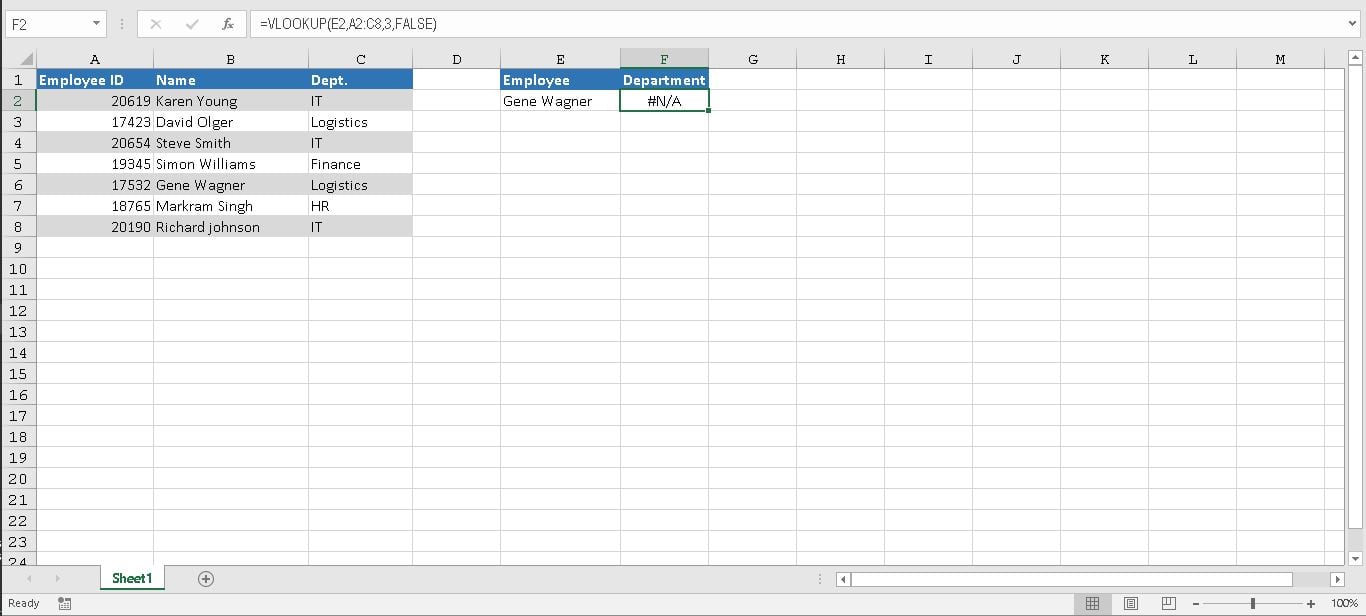
The #N/A error results because the lookup value “Gene Wagner” appears in the second column (Name) of the table array argument A2:C8. In this case, Excel is looking for it in column A, not column B.
The #N/A error can be resolved using one of the following fixes.
Changing the table array reference
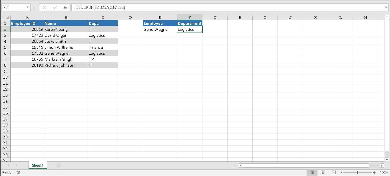
You can fix the #N/A error adjusting your VLOOKUP to refer the correct column. If that’s not possible, try to move the columns. But that might be impractical when you have a large dataset or maybe there are other logical reasons why you can’t move the columns. We can set the table array to B2:C8 which makes our formula
=VLOOKUP(E2,B2:C8,2,FALSE)
Using the CHOOSE function with VLOOKUP in an Array formula
You can use VLOOKUP with the CHOOSE function to create an Array formula which would look up E2 in B2:B8 and return a result from C2:C8 if successful. You would need to apply this formula using CTRL + SHIFT + ENTER. The formula will be
=VLOOKUP(E2,CHOOSE({1,2},B2:B8, C2:C8),2,0)

Limitations of the VLOOKUP function
There are certain limitations using VLOOKUP. Besides the lookup value in the first column, VLOOKUP needs the return a value in the specified range. You have to know the column number containing the return value. This can be very inefficient when you have a large table.
VLOOKUP makes a static reference to the table, so adding a new column to the table breaks the VLOOKUP formula. VLOOKUP will only look for a closest or exact match to a value. It also assumes by default that the first column in the table array is sorted alphabetically.
If your table is not sorted that way, VLOOKUP will return the first closest match which in many cases may not be your desired output. For these reasons, the best alternative for a VLOOKUP is a combination of INDEX/ MATCH functions.
Using a combination of INDEX and MATCH functions
Using a combination INDEX and MATCH, we can find a matching value when the lookup value is not on the first column of the table array. INDEX() returns the value of a cell in a table based on the column and row number. MATCH() returns the position of a cell in a row or column.
Combining these two functions we can look up a value both horizontally and vertically. The combination of INDEX and MATCH overcomes the limitations of VLOOKUP. INDEX and MATCH don’t require the return value to be in the same column as the lookup column. You can specify either a row or a column as an array- or specify both. The lookup value doesn’t have to be on the first column with INDEX and MATCH; it can be anywhere.
INDEX and MATCH offer the flexibility of making dynamic reference to the column which contains the return value; we can add columns to your table without breaking the formula. INDEX and MATCH offer more options for matches. You can specify an exact, greater than or lesser than match.
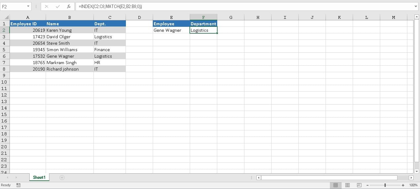
Back to our employee records example. To implement the combination of INDEX and MATCH, we will assign the formula =INDEX(C2:C8,MATCH(E2,B2:B8,0)) to cell F2. This will return the Department for “Gene Wagner” which is “Logistics.”
Finding matching value in your own data set can be more complex, and you might need to use techniques other than those listed above. If you are in a rush and want your problem answered by an Excel expert, try our service. The experts are available to help you 24/7 at the link to the right. The first question is free.


Leave a Comment