

We use drop-down lists in the Google sheet to enter data from a predefined list of items. In this tutorial, we will explore the ways to create or modify a drop-down menu using an Excel data validation list based on a named range, range of cells, list of values and a dynamic drop-down. We will also learn how to create a dropdown in one workbook and move it to a different workbook.
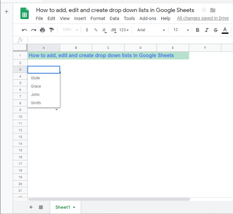 Figure 1 – How to make a dropdown in google sheets
How to add a drop-down menu in google sheet
- We will open a new Google spreadsheet
- Next, we will select the cells where we want to add our drop-down list
- Now we will click Data, then Data validation
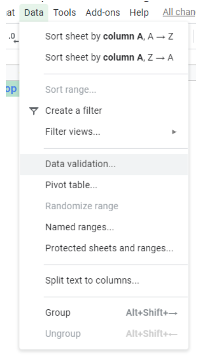 Figure 2 – Google sheets data validation
- In the Criteria option, we will select either:
- List of items: Enter items using commas with no space
- List from the range: Select cells that will be included in the list
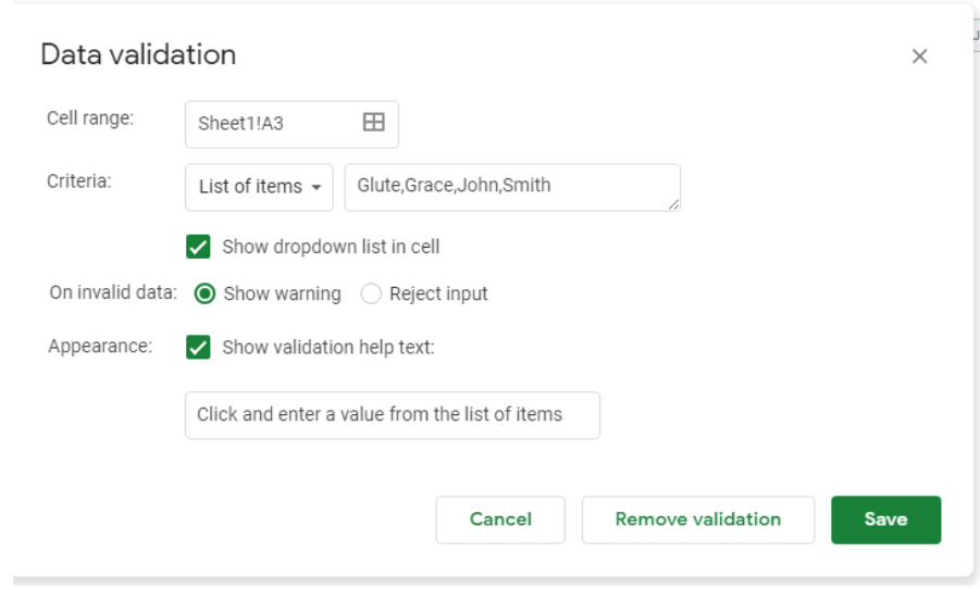 Figure 3 – Dropdown list using a list of items
- Next, the cells will now have a down arrow. If we wish to remove the arrows, we will uncheck “show the dropdown list in cell”.
 Figure 4 – Google sheets drop down box
- Lastly, we will click save.
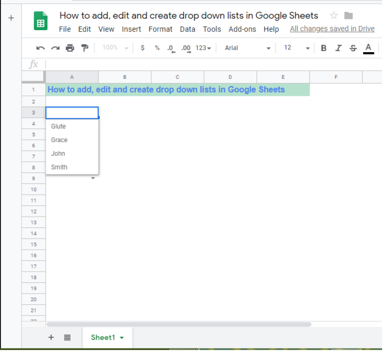 Figure 5 – Make a dropdown list in google sheets
Creating a Google sheet drop-down list based on a named range
Suppose we have an entry of ingredients we need some time in the future, we may:
- Sort Entries first in the manner we want them to appear in the future
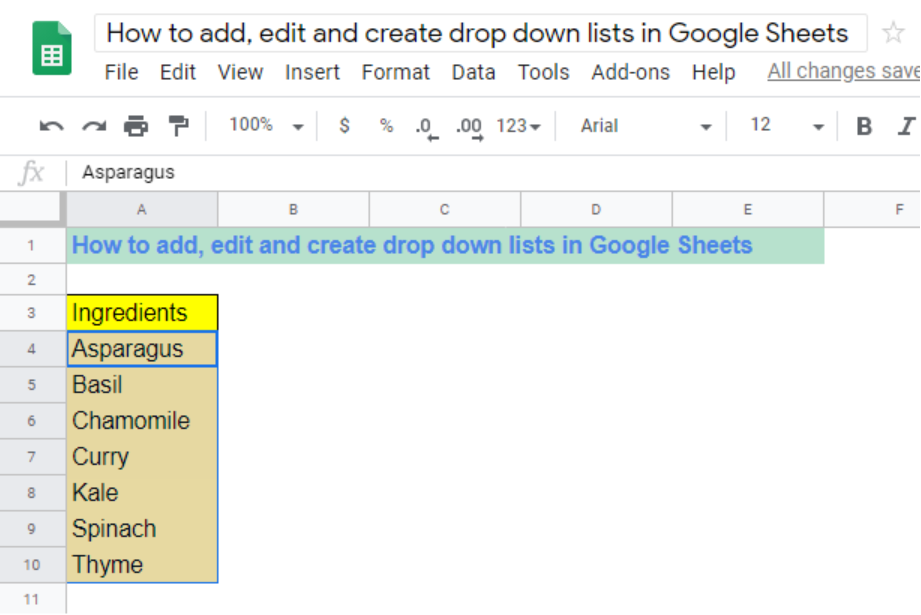 Figure 6 – Google sheets numbered list
- Next, we will create a named range by selecting all entries and right-clicking. Then we will go to the Formula Tab and tap Name Manager.
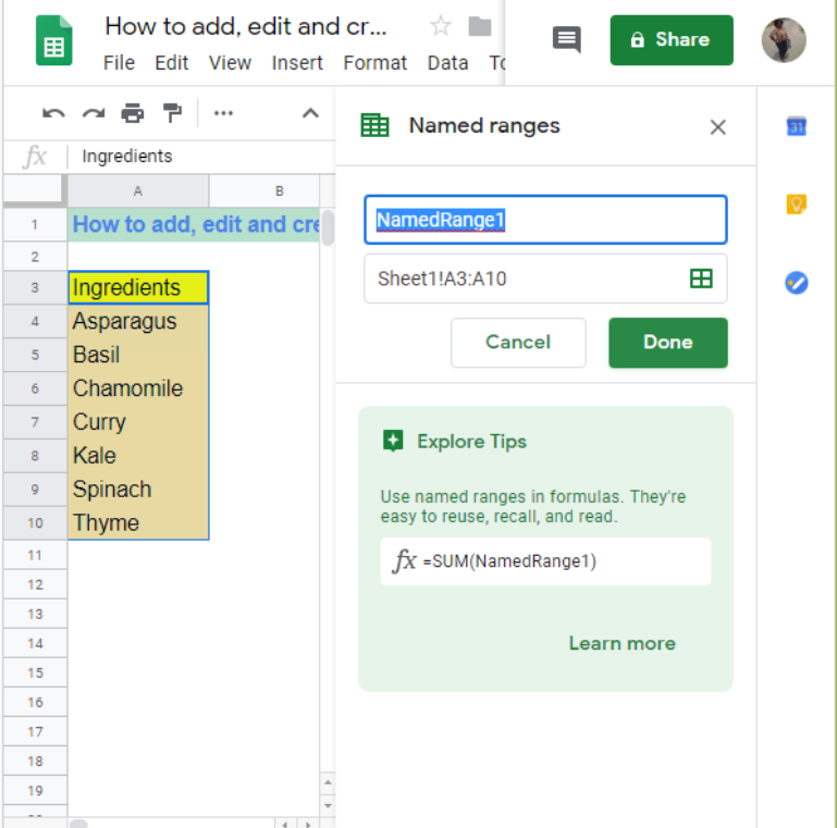 Figure 7 – Insert cell reference for making google sheet dropdown list
- In the Name Manager dialog, we will click New, and type desired name for entries. Check that range is correct as displayed in the refers box and click OK.
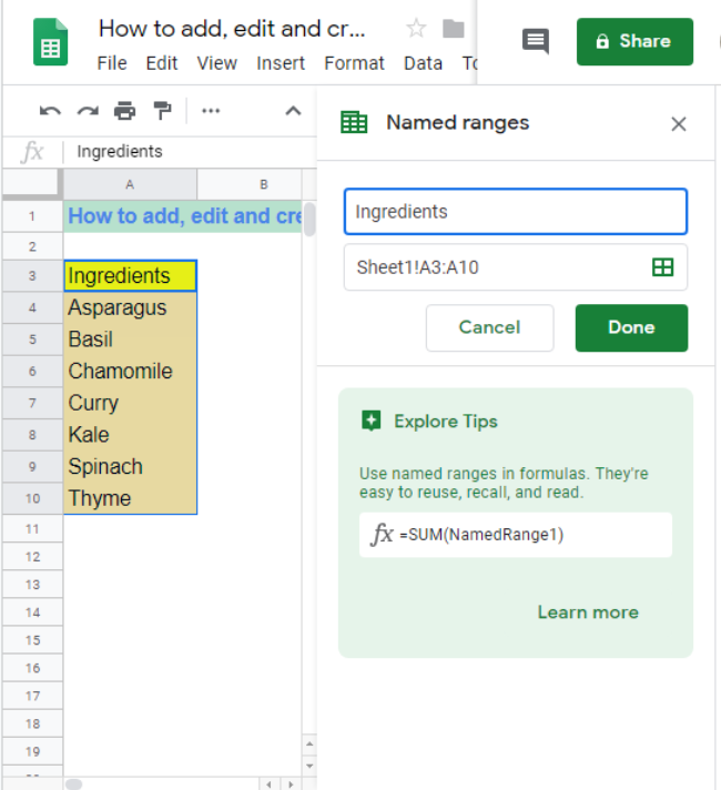 Figure 8 – Google sheets lists based on named range
- We will pick a location for our new drop-down list by selecting an entire column or a range of cells. We can equally click on a single cell wherever we want the list to appear
- Next, we will go to the Data Tab, click Data Validation and go to the Settings Tab
- In the settings tab, we select Allow under List and in the Source box, we will type the name for our list.
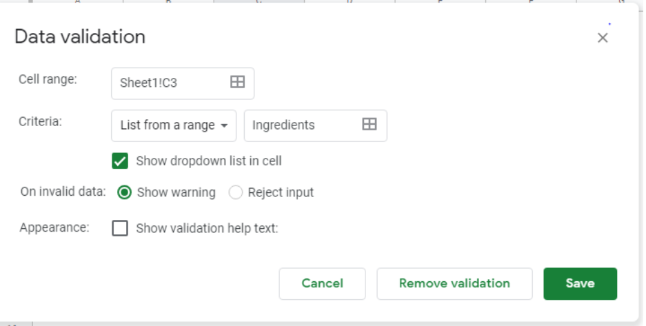 Figure 9 – Data validation based on a named range
- Now we will check that the In-cell dropdown is checked and select OK.
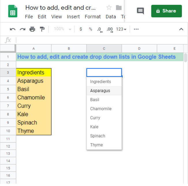 Figure 10 – Add a dropdown to google sheet
How to change or delete drop-down list in Google Sheet
- We will open the Google Spreadsheet
- Next, we will select the cells we wish to change
- Now click Data and Data validation
- To change options, we will go to Criteria and choose to edit the items
- If we wish to delete a list, then we will click “Remove validation” and select Save
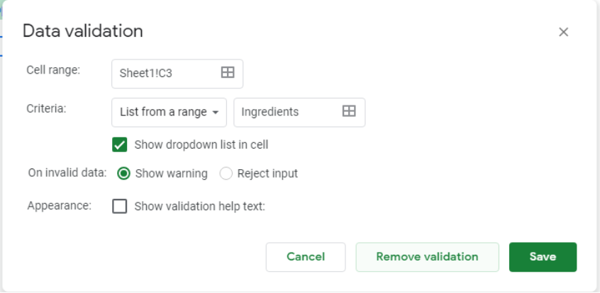 Figure 11 – Changing the dropdown menu in google sheets
How to add values to a drop-down list automatically
Typically, when we will want to add new values to our pre-existing drop-down list in the future, we will be met with a Warning option which is ticked off, when invalid data is entered. Due to this warning, the new entry will not be saved and we may find an orange notification at the corner of the cell. In this event, it is important to create an automatically filled drop-down list. This ensures that our contents be stored automatically right after we input it into a cell.
- We will go to the Spreadsheet that contains our drop-down list and copy cells to a different column in the same sheet.
- Next, we will change the dropdown list settings for specified range by selecting cells, clicking data and then data validation to change range criteria for the new column created.
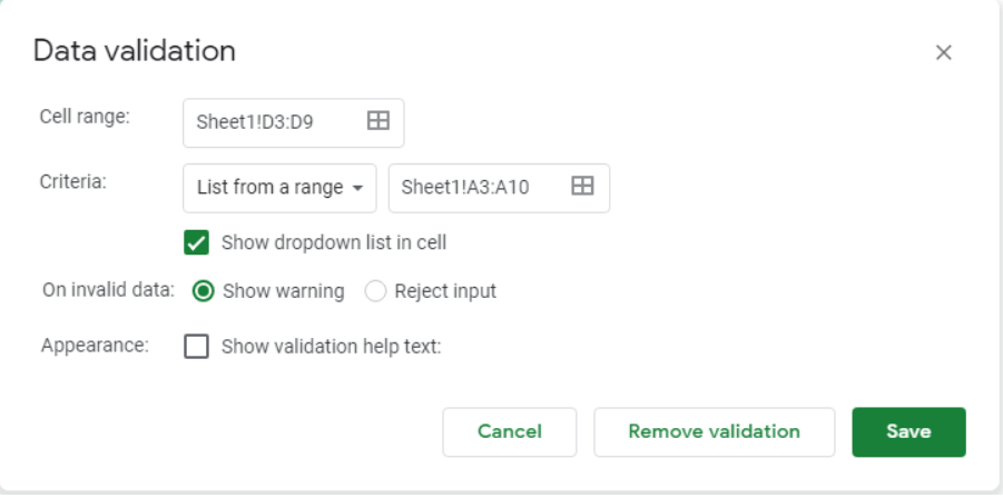 Figure 12 – Dynamic dropdown list google sheets
- Next, we will save changes
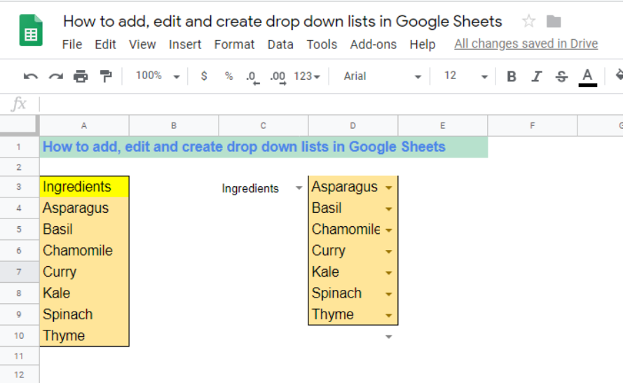 Figure 13 – Google sheets dependent dropdown list
How to make a dynamic automatically updated Google Sheet dropdown list
- First, we will create a dropdown based on the named range as described in an earlier session
- Next, when creating the name, we put in this formula in the Refers to box
=OFFSET(Sheet1!$A$1,0,0,COUNTA(Sheet1!$A:$A),1)
Where:
- Sheet1 – the name of the sheet
- A – the column where our drop-down list is located.
- $A$3 – the cell containing the first item of the drop-down list
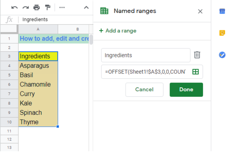 Figure 14 – Updating cell values based on the selection in the dropdown list
Make a drop-down list from another Google sheet workbook
To create a drop-down menu from another workbook, we will need 2 named ranges, one in our source workbook and the other wherever we wish to have our Excel Data Validation list. In this process, we may have two kinds of drop-down lists depending on our approach.
Creating a static dropdown list from another workbook
With this kind of drop-down list, we cannot update, add or remove entries in the source list automatically but must modify the source list manually.
- We will open the workbook with the source list and create a named range for entries we want in the drop-down list
- Next, we will open the new workbook and create a name that references the source list
- In our main workbook, we have to select the cells for the dropdown list, click Data, tap Data Validation and enter the name we created in the second step in the source box. Lastly, we will tap, OK.
A dynamic Dropdown list from another workbook
- We will create a named range in the sourcebook, using the OFFSET formula explained in the creating dynamic drop-down section
- In the main workbook, we apply data validation in our usual way.
Explanation
When we frequently create lists with repeated values, it is excellent to avoid misspelled entries by creating a list that can be used at any time to make new datasheets. By creating a Google sheet drop-down filter, we reduce the time and error involved in entering the same value over again.
The OFFSET function
We use the OFFSET function to take a number and return with the reference to the range that includes non-empty cells.
The COUNTA function
The COUNTA function will count all non-empty cells in the column specified by the OFFSET function.
Notes
When we enter data in a cell that does not match the items in our list, we will receive a warning. If we want to allow users to only enter items on the list. Then we go to “On Invalid data” and mark “Reject input”.
Instant Connection to an Expert through our Excelchat Service
Most of the time, the problem you will need to solve will be more complex than a simple application of a formula or function. If you want to save hours of research and frustration, try our live Excelchat service! Our Excel Experts are available 24/7 to answer any Excel question you may have. We guarantee a connection within 30 seconds and a customized solution within 20 minutes.


Leave a Comment