

DVAR is a database function in Excel that returns the variance of a population by using the samples that match the given criteria. This tutorial will assist all levels of Excel users in the usage and syntax of DVAR function.
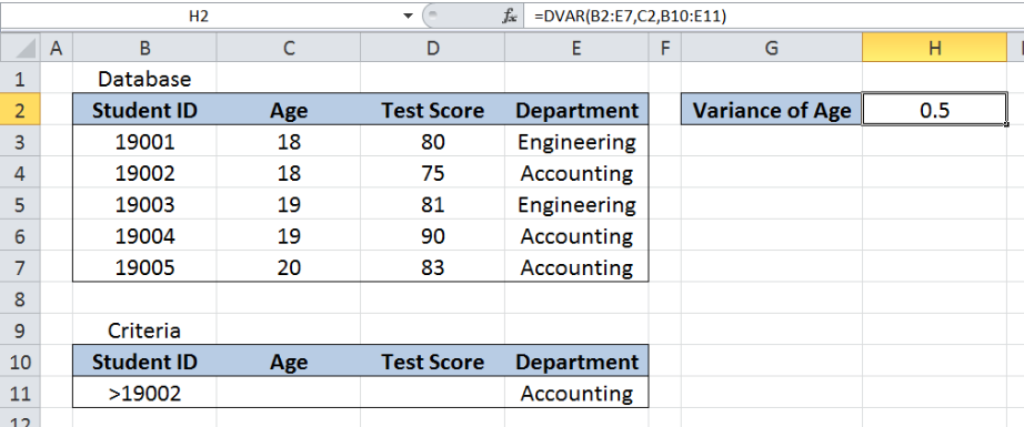 Figure 1. Final result of the DVAR function
Final formula: =DVAR(B2:E7,C2,B10:E11)
Syntax of the DVAR Function
=DVAR(database, field, criteria)
- Database – The range of cells containing our data
- Field – The column header which represents the field whose variance we want to calculate; can be entered as text enclosed in double quotation marks, as a number corresponding to the column number, or as a cell reference
- Criteria – the range of cells containing the conditions that we specify
Setting up our Data
Our data consists of four columns : Student ID (column B), Age (column C), Test Score (column D) and Department (column E). The range for the database is B2:E7. The criteria range is B10:E11. The database and criteria ranges should have matching headers.
In cell H2, we want to determine the variance of Age for the criteria we specify. Variance is simply the square of the standard deviation, and it measures how far each value in the dataset is from the mean.
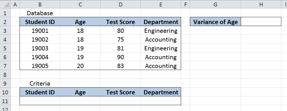 Figure 2. Sample data for the DVAR function
Variance of Age for Accounting Students using DVAR
We want to calculate the variance of the age of Accounting students in the list by using the DVAR function. Let us follow these steps:
Step 1. Enter “Accounting” in cell E11
Step 2. Select H2 and enter the formula: =DVAR(B2:E7,C2,B10:E11)
Step 3. Press ENTER
The range for the database is B2:E7. The criteria range is B10:E11. The field is C2, which is the cell reference to Age. The field value can also be entered as “Age” instead of C2.
The result in cell H2 is 1.0, which is the variance for the age of Accounting students.
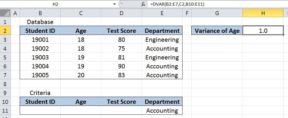 Figure 3. Entering the formula for DVAR function
The DVAR function can handle more than one criteria. Suppose we want to find the variance of the age of Accounting students with Student ID greater than 19002. We follow these steps:
Step 1. Enter “Accounting” in cell E11
Step 2. Enter “>19002” in cell B11
Step 3. Select H2 and enter the formula: =DVAR(B2:E7,C2,B10:E11)
Step 4. Press ENTER
The formula is still the same as in the previous example. This time, there is one criteria added “>19002” for Student ID. As a result, the DVAR formula returns 0.5 in cell H2, which is the variance of the age of Accounting students with Student ID greater than 19002.
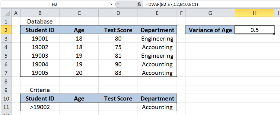 Figure 4. Using DVAR to find the variance of age based on the given criteria
Most of the time, the problem you will need to solve will be more complex than a simple application of a formula or function. If you want to save hours of research and frustration, try our live Excelchat service! Our Excel Experts are available 24/7 to answer any Excel question you may have. We guarantee a connection within 30 seconds and a customized solution within 20 minutes.


Leave a Comment