

Excel allows a user to count values with multiple criteria and or logic using the COUNTIFS and SUM functions. This step by step tutorial will assist all levels of Excel users in creating a COUNTIFS with multiple criteria and or logic.
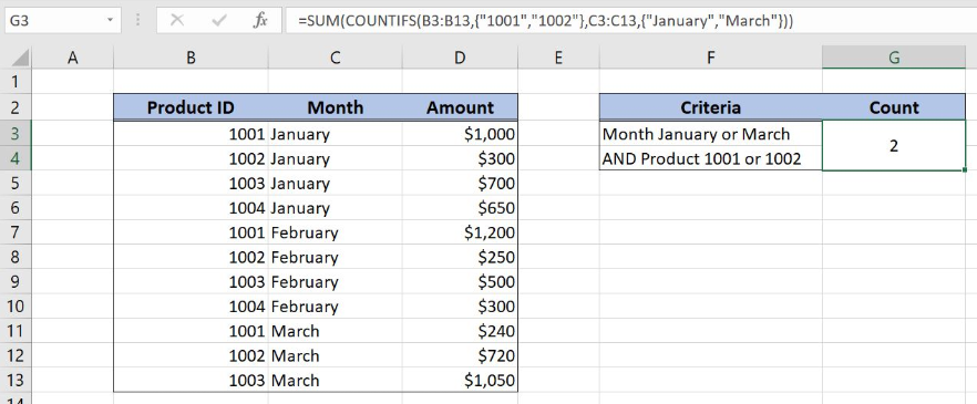 Figure 1. The result of the formula
Syntax of the COUNTIFS Formula
The generic formula for the COUNTIFS function is:
=COUNTIFS(criteria_range1, criteria1, criteria_range2, criteria2, ... )
The parameters of the COUNTIFS function are:
- criteria_range1, criteria_range2 – ranges where we want to apply our criteria
- criteria1, criteria2 – a criteria in criteria ranges which we want to count.
Syntax of the SUM Formula
The generic formula for the SUM function is:
=SUM(number1, number2, …, numberN)
The parameters of the SUM function are:
- number1, number2, …, numberN – numbers which we want to sum.
Setting up Our Data for the Formula
In the first data table, we have 3 columns: “Product ID” (column B), “Month” (column C) and “Amount” (column D). In the cells F3 and F4 we have criteria for counting. We want to count items which have the month January or March and Product ID 1001 or 1002. The results will be in the cell G3.
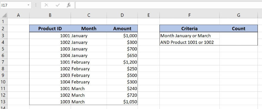 Figure 2. Data that we will use in the example
Count Items with Multiple Criteria and Or Logic
In our example, we want to count items which have the month January or March and Product ID 1001 or 1002.
The formula looks like:
=SUM(COUNTIFS(B3:B13, {"1001", "1002"}, C3:C13, {"January", "March"}))
The parameter criteria_range1 is B3:B13 and the criteria1 is the array {“1001”, “1002”}. The parameter criteria_range2 is C3:C13 and the criteria2 is {“January”, “March”}. The result of this COUNTIFS function is 2 numbers, which are number parameters of the SUM function.
To apply the formula, we need to follow these steps:
- Select cell G3 and click on it
- Insert the formula:
=SUM(COUNTIFS(B3:B13,{"1001","1002"},C3:C13,{"January","March"})) - Press enter.
 Figure 3. Counting items with multiple criteria and or logic
As you can see, we have two items meeting both criteria. In row 3, the Product ID is 1001 and the month is January and in row 12 we have the Product ID 1002 and the month March. Therefore, the SUM function sums these two items and the result in G3 is 2.
Most of the time, the problem you will need to solve will be more complex than a simple application of a formula or function. If you want to save hours of research and frustration, try our live Excelchat service! Our Excel Experts are available 24/7 to answer any Excel question you may have. We guarantee a connection within 30 seconds and a customized solution within 20 minutes.


Leave a Comment