Summary Count with Percentage Breakdown

While working with Excel, we are able to obtain the count per specified criteria and present the breakdown in percentage form by using the COUNTIF and COUNTA functions.  COUNTIF returns the number of values in a specified range based on a given condition while COUNTA returns the number of non-empty cells in a range.  

This step by step tutorial will assist all levels of Excel users in obtaining the summary count with percentage breakdown.  

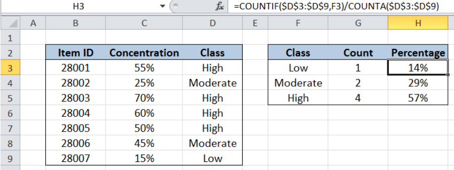Figure 1. Final result: Summary count with percentage breakdown

Final formula: =COUNTIF($D$3:$D$9,F3)/COUNTA($D$3:$D$9)

Syntax of COUNTIF Function

=COUNTIF(range,criteria)

Parameters:

• range – the data range that will be evaluated using the criteria
• criteria – the criteria or condition that determines which cells will be counted

Syntax of COUNTA Function

=COUNTA(value1, [value2], ...)

Parameters:

• value1 –  any value that we want to count
• Only value1 is required; succeeding values are optional  

Setting up Our Data

Our table contains a list of Item ID (column B), Concentration (column C) and Class (column D).  Cells F3:F5 contains our criteria which lists the classes Low, Moderate and High. Cells G3:G5 contains the count of each class.  In cells H3:H5, we will determine the percentage breakdown of the classes based on their count.

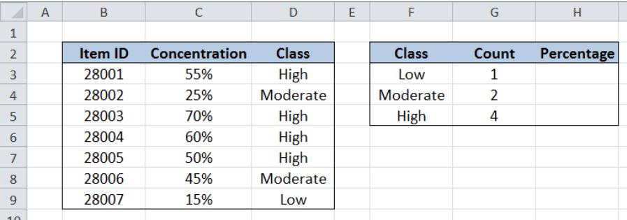Figure 2. Sample data to get summary count with percentage breakdown

Summary count with percentage breakdown

To get the summary count of each class and present the percentage breakdown, we follow these steps:

Step 1.  Select cell H3

Step 2.  Enter the formula: =COUNTIF($D$3:$D$9,F3)/COUNTA($D$3:$D$9)

Step 3: Press ENTER

Step 4: Copy the formula in cell H3 to cells H4 and H5 by clicking the “+” icon at the bottom right-corner of cell H3 and dragging it down.  

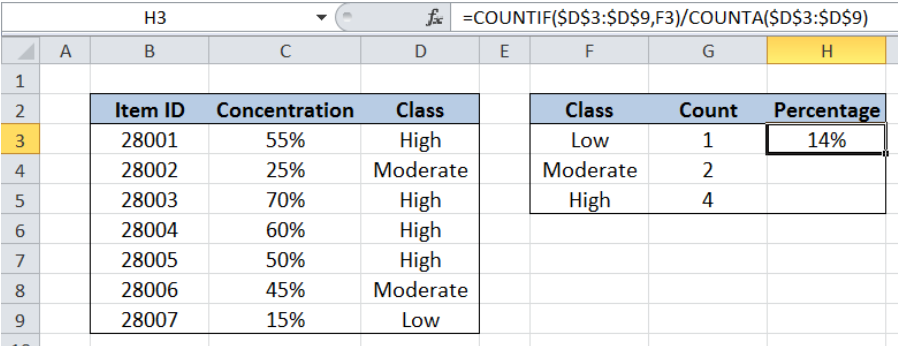Figure 3. Entering the formula to get percentage breakdown of “Low” class

The range for our data set is D3:D9, which contains the “Class”. The dollar symbols “$” fix the cells so that we can easily copy and paste the formula to other cells.  The criteria is F3 or “Low”, which is the class that we want to summarize.

Our formula first counts the values with “Low” class, then counts the number of values under the column “Class”.  The two values are then divided. As a result, our formula returns the percentage breakdown of the class “Low”, which is 14%.  

Copying the formula to cells H4 and H5 returns the values 29% and 57%, which are the percentage breakdown for the classes “Moderate” and “High”, respectively.  

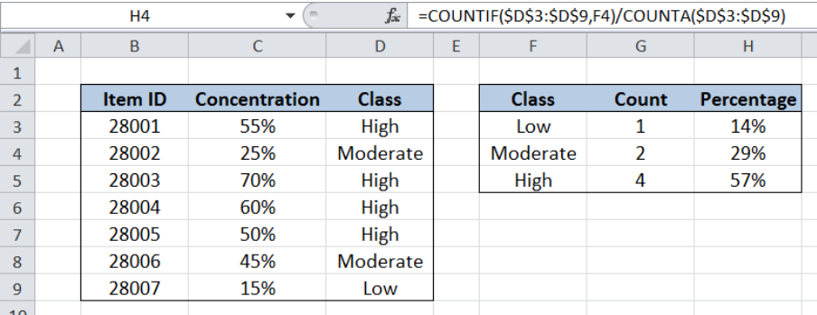Figure 4. Using COUNTIF and COUNTA to get summary count with percentage breakdown

Most of the time, the problem you will need to solve will be more complex than a simple application of a formula or function. If you want to save hours of research and frustration, try our live Excelchat service! Our Excel Experts are available 24/7 to answer any Excel question you may have. We guarantee a connection within 30 seconds and a customized solution within 20 minutes.