

Excel allows a user to compare two columns by using the SUMPRODUCT function. As a result, we get a number of matches between two columns. This step by step tutorial will assist all levels of Excel users in counting matches between two columns.
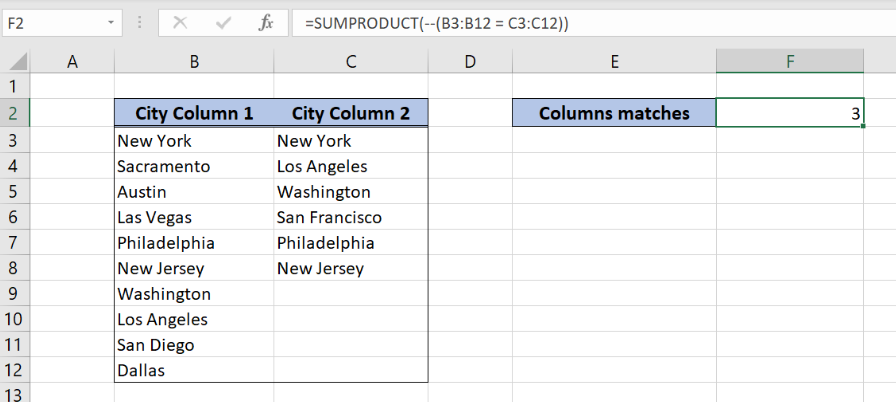 Figure 1. The result of the SUMPRODUCT function
Syntax of the SUMPRODUCT Formula
The generic formula for the SUMPRODUCT function is:
=SUMPRODUCT(--(array1 = array2))
The parameters of the SUMPRODUCT function are:
- array1 and array2 – range of cells that we want to compare. The arrays must be the same size.
The function compares cells one by one and returns Booleans TRUE or FALSE. Using the double negation “–” in front of the logical test, the Booleans are converted to 1 or 0. At the function sums everything and returns a result.
Setting up Our Data for the SUMPRODUCT Function
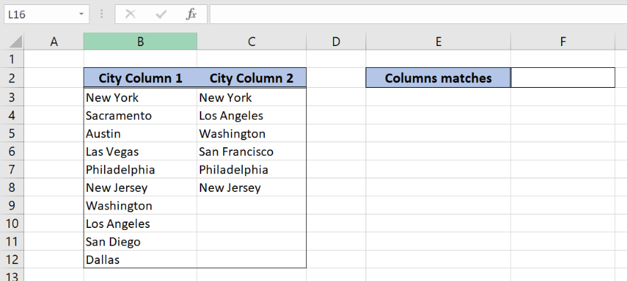 Figure 2. Data that we will use in the SUMPRODUCT example
In columns B and C we have two lists of cities which we want to compare. In the cell F2, we want to return the total number of matches between two columns.
Using the SUMPRODUCT to Count Matches Between Two Columns
In our example, we want to check if cells from column B and column C are the same, and count matches in F2.
The formula looks like:
=SUMPRODUCT(--(B3:B12 = C3:C12))
The array1 is B3:B12 and array2 is C3:C12. Let’s evaluate the formula and see the result:
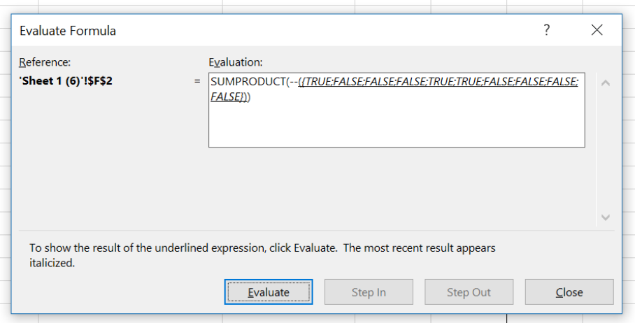 Figure 3. Evaluate the SUMPRODUCT function
As you can see, the function has TRUE if cells are equal or FALSE if not. Rows 1, 6 and 7 are the same, so in the function we have TRUE for these cells. FInally these 3 values are summed and we have the result 3 in the cell F3.
To apply the SUMPRODUCT function, we need to follow these steps:
- Select cell F2 and click on it
- Insert the formula:
=SUMPRODUCT(--(B3:B12 = C3:C12)) - Press enter
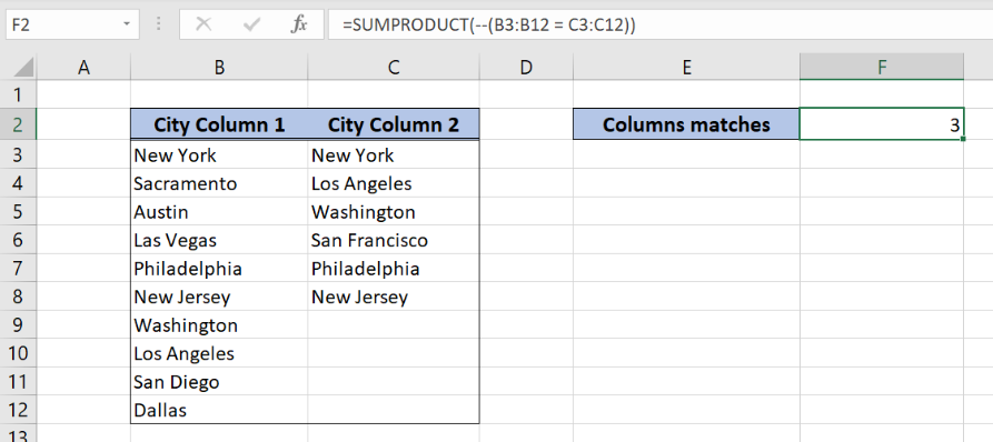 Figure 4. Using the SUMPRODUCT to count matches between two columns
Most of the time, the problem you will need to solve will be more complex than a simple application of a formula or function. If you want to save hours of research and frustration, try our live Excelchat service! Our Excel Experts are available 24/7 to answer any Excel question you may have. We guarantee a connection within 30 seconds and a customized solution within 20 minutes.


Leave a Comment