

Excel allows a user to count rows if multiple criteria are met by using the SUMPRODUCT function. This step by step tutorial will assist all levels of Excel users in counting rows that meet multiple criteria.
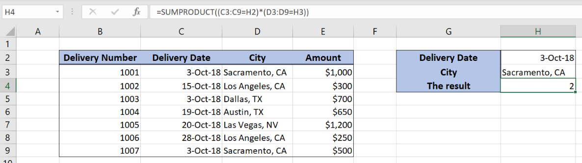 Figure 1. The result of the SUMPRODUCT function
Syntax of the SUMPRODUCT Formula
The generic formula for the SUMPRODUCT function is:
=SUMPRODUCT((array1 = condition1) * (array2 = condition2))
The parameters of the SUMPRODUCT function are:
- array1 and array2 – range of cells where we want to apply a condition
- condition1 and condition2 – conditions which we want to apply on arrays.
The function compares cells one by one and returns Booleans TRUE or FALSE for both arrays. In the end, it multiplies Booleans and sums the results.
Setting up Our Data for the SUMPRODUCT Function
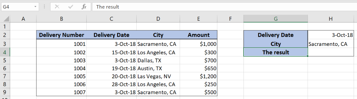 Figure 2. Data that we will use in the SUMPRODUCT example
Let’s look at the structure of the data we will use. The table consists of 4 columns: “Delivery Number” (column B), “Delivery Date” (column C), “City” (column D) and “Amount” (column E). In the cell H4, we want to get the count of all the rows that meet two conditions. The first condition is Delivery Date equal to H2, while the second is City equal to H3.
Using the SUMPRODUCT to Count Rows Meeting Two Criteria
In our example, we want to count all rows where the delivery date is 3-Oct-18 and City is Sacramento, CA.
The formula looks like:
=SUMPRODUCT((C3:C9 = H2) * (D3:D9 = H3))
The array1 is C3:C9 and condition1 is H2. The array2 is D3:D9 and condition2 is H3. Let’s evaluate the formula and see the result:
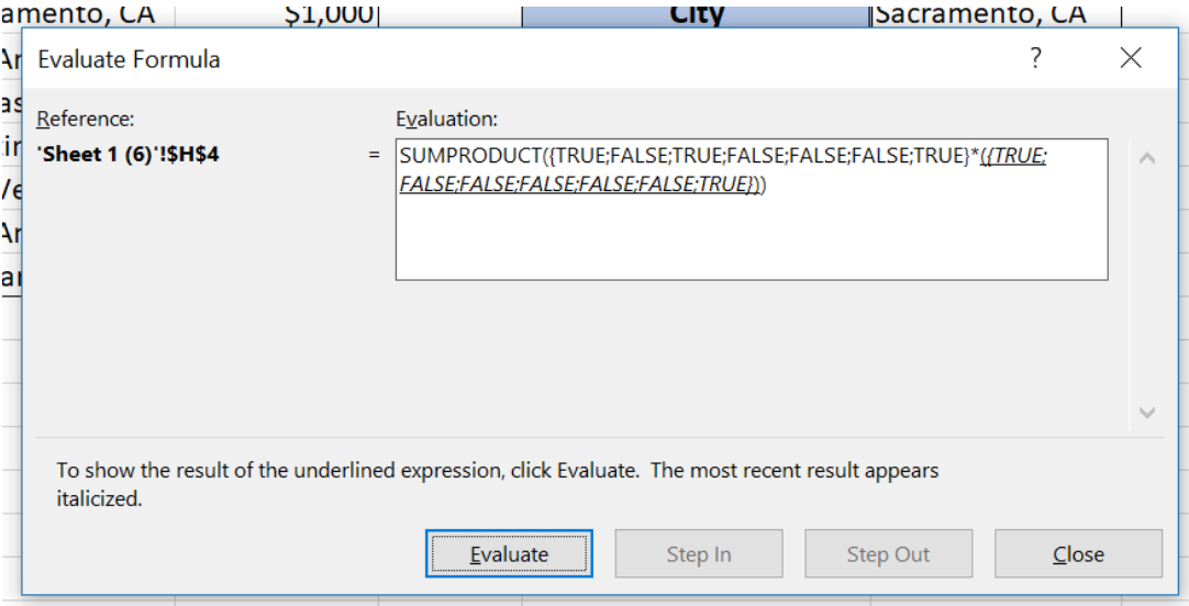 Figure 3. Evaluate the SUMPRODUCT function
As you can see, the function has TRUE if conditions are met or FALSE if not. The first part of the function returns {TRUE; FALSE; TRUE; FALSE; FALSE; FALSE; TRUE}. The second part returns {TRUE; FALSE; FALSE; FALSE; FALSE; FALSE; TRUE}.
After this multiplies these values one by one, where TRUE is 1 AND FALSE 0. The result of the multiplication is: {1, 0, 0, 0, 0, 0, 1}. In the end, all the values are summed and the result in the cell H4 is 2.
To apply the SUMPRODUCT function, we need to follow these steps:
- Select cell H4 and click on it
- Insert the formula:
=SUMPRODUCT((C3:C9 = H2) * (D3:D9 = H3)) - Press enter
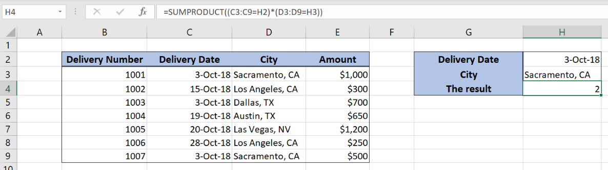 Figure 4. Using the SUMPRODUCT to count rows meeting two criteria
Most of the time, the problem you will need to solve will be more complex than a simple application of a formula or function. If you want to save hours of research and frustration, try our live Excelchat service! Our Excel Experts are available 24/7 to answer any Excel question you may have. We guarantee a connection within 30 seconds and a customized solution within 20 minutes.


Leave a Comment