How to count cells containing either a or b

Excel allows a user to count cells in a range which contains one of the selected words using the SUMPRODUCT, ISNUMBER and FIND functions. This step by step tutorial will assist all levels of Excel users to count cells that contain either a or b.

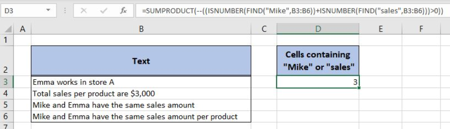Figure 1. The result of the formula

Syntax of the SUMPRODUCT Formula

The generic formula for the SUMPRODUCT function is:

=SUMPRODUCT(--(array))

The parameter of the SUMPRODUCT function is:

array – an array of values which we want to sum. The double minus before the array converts TRUE to 1 and FALSE to 0.

Syntax of the ISNUMBER Formula

The generic formula for the ISNUMBER function is:

=ISNUMBER(value)

The parameter of the ISNUMBER is:

value – a value which we want to check if it’s a number or not.

If the value is numeric, the function returns TRUE and if it’s not FALSE.

Syntax of the FIND Formula

The generic formula for the FIND function is:

=FIND(find_text, within_text, [start_num])

The parameters of the FIND function are:

find_text – a text which we want to find in another text

within_text -a text where we want to find a find_text

[start_num] -a position from which we want to search for a find_text. This parameter is optional. If it’s omitted, the function will search from the beginning.

If a find_text is found, the function returns the beginning position in a text. If it’s not found, the function returns an error. Note that the FIND function is case-sensitive.

Setting up Our Data for the Formula

Let’s look at the structure of the data we will use. In column B (“Text”), we have texts where we want to count cells containing “Mike” or “sales”. In column D (“Cells containing “Mike” or “sales”), we want to get a result.

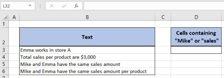Figure 2. Data that we will use in the example

Counting Cells Containing at Least One of Two Selected Words

In our example, we want to check how many cells contain “Mike” or “sales”. The result will be in the cell D3.

The formula looks like:

=SUMPRODUCT(--((ISNUMBER(FIND("Mike",B3:B6))+ISNUMBER(FIND("sales",B3:B6)))>0))

The parameter find_text of the first FIND function is “Mike” while the within_text is B3:B6 range. The result of this function is the array, which is the value parameter of the ISNUMBER function.

The find_text of the second FIND function is “sales” while the within_text is B3:B6 range. The result of this function is the array, which is the value parameter of the ISNUMBER function.

The results of two ISNUMBER functions are two arrays which are summed and present the parameter of the SUMPRODUCT function.

To apply the formula, we need to follow these steps:

Select cell D3 and click on it
Insert the formula: =SUMPRODUCT(--((ISNUMBER(FIND("Mike",B3:B6)) + ISNUMBER(FIND("sales",B3:B6)))>0))
Press enter.

The FIND function looks for the word and returns the first position of a word or an error. If we evaluate this function we can see the following array:

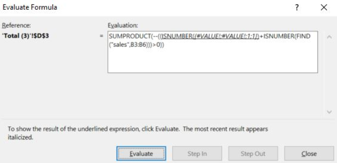Figure 3. Evaluate the formula

In the first two cells, “Mike” is not found, and in the third and fourth it starts from the first position. Therefore, the array is {#VALUE!; #VALUE!; 1; 1}.

Now the ISNUMBER converts these values to TRUE and FALSE. Therefore, the result of the ISNUMBER function is the array {FALSE, FALSE, TRUE, TRUE}.

Similarly, the function executes the second FIND and ISNUMBER functions and the array is {FALSE, TRUE, TRUE, TRUE}. As we can see, the word “sales” occurs in cells B4, B5 and B6.

Now, these two arrays are summed, as we can see in Figure 4.

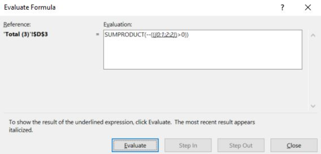Figure 4. Evaluate the formula

We can see that FALSE+FALSE gives 0, TRUE+FALSE 1 and TRUE+TRUE 2. Finally, we need to check which of array values are greater than 0. After that, the array is {FALSE, TRUE, TRUE, TRUE}.

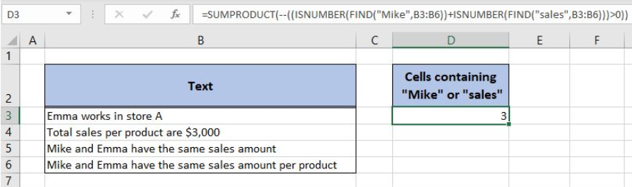Figure 5. Using the formula to count cells containing either “Mike” or “Sales”

Finally, the SUMPRODUCT converts TRUE and FALSE to 1 and 0, so the array is {0, 1, 1,1}. The sum of this array is 3, which means that the words “Mike” or “sales” occur in 3 cells. Therefore, the result in D3 is 3.

Most of the time, the problem you will need to solve will be more complex than a simple application of a formula or function. If you want to save hours of research and frustration, try our live Excelchat service! Our Excel Experts are available 24/7 to answer any Excel question you may have. We guarantee a connection within 30 seconds and a customized solution within 20 minutes.