Shade alternating groups of n rows

When we want to shade every n rows in excel, we can use a formula that is based on ROW, CEILING and ISEVEN functions together with conditional formatting. This article provides a clear guide on how you can shade alternating groups of n rows while working in excel.

Figure 1: Shading every n rows in excel

General syntax of the formula

=ISEVEN(CEILING(ROW() –offset, n)/n)

Where;

• n- is the number of rows in a group
• offset- is the number used to normalize the first row

How this formula works

This formula is composed of three functions, and they play the following functions:

• ROW function- this is used to normalize the row numbers to start with 1
  ROW() – offset
  Notice that the first row of our data in the figure above is in row 6, so we can use an offset of 5.

• The result of the ROW function goes to the CEILING function. This function is responsible for rounding incoming numbers up to a specified multiple of n.

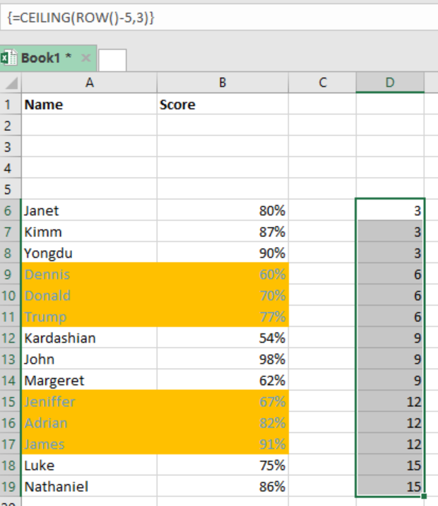Figure 2: Example of how to shade alternating rows in excel

• Now to count by groups of n, which in our case is 3, the count above is divided by n, 3, starting with 1 as illustrated below;

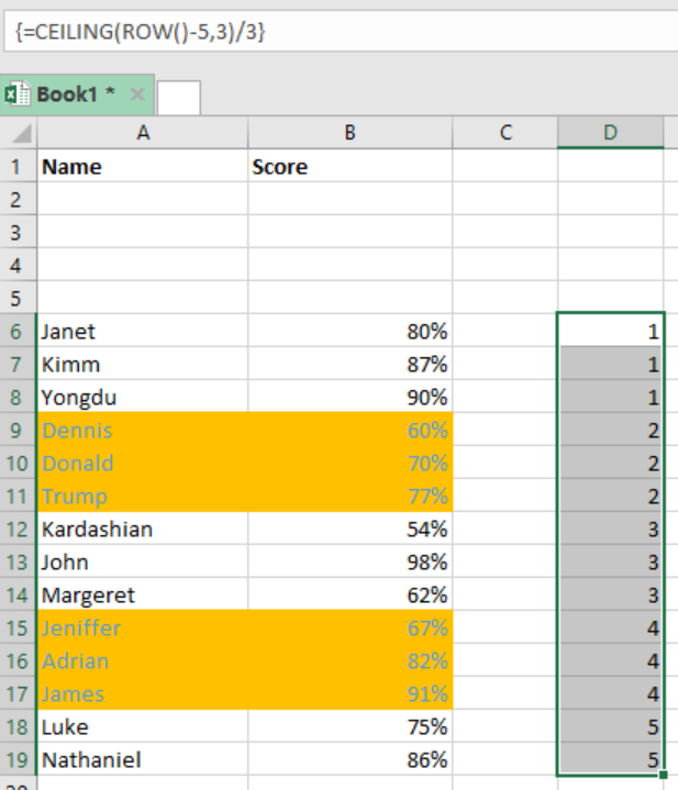Figure 3: Illustration of how to shade alternating groups in excel

The conditional formatting is the triggered by the ISEVEN function which forces a TRUE for all the even rows in the groups. For those that are not even, the conditional formatting is not triggered, therefore, they do not change.

How to shade first group

Instead of starting with the second, you can as well shade the first group of n rows. All you need to do is to replace the ISEVEN function with its ISODD counterpart. The formula with the example below;

=ISODD(CEILING(ROW() –offset,n/n)

Example

Figure 4: How to shade odd rows in excel

In this particular example, we have shaded all odd rows. To do this, proceed as follows;

• Step 1: Provide the data in the table
• Step 2: Highlight the entire data and apply conditional formatting.
• Step 3: While formatting, apply the formula =ISODD(CEILING(ROW()-5,3)/3)
• Step 4: Press “Apply and the “Ok” to apply the conditional formatting.

Instant Connection to an Expert through our Excelchat Service

Most of the time, the problem you will need to solve will be more complex than a simple application of a formula or function. If you want to save hours of research and frustration, try our live Excelchat service! Our Excel Experts are available 24/7 to answer any Excel question you may have. We guarantee a connection within 30 seconds and a customized solution within 20 minutes.