How to Apply Conditional Formatting Between Sheets in Excel

Excel Conditional Formatting can be used to match values in different cells along with reconciliation of data. Final result is as follow:

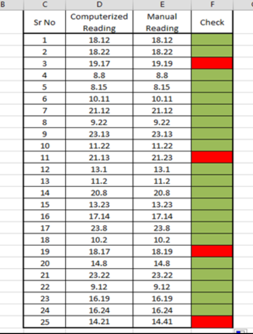Figure 1 – Final Result

Our data-set show readings extracted from computer system and values manually note down. Our goal here is to check if values extracted from computer and the manual values match.

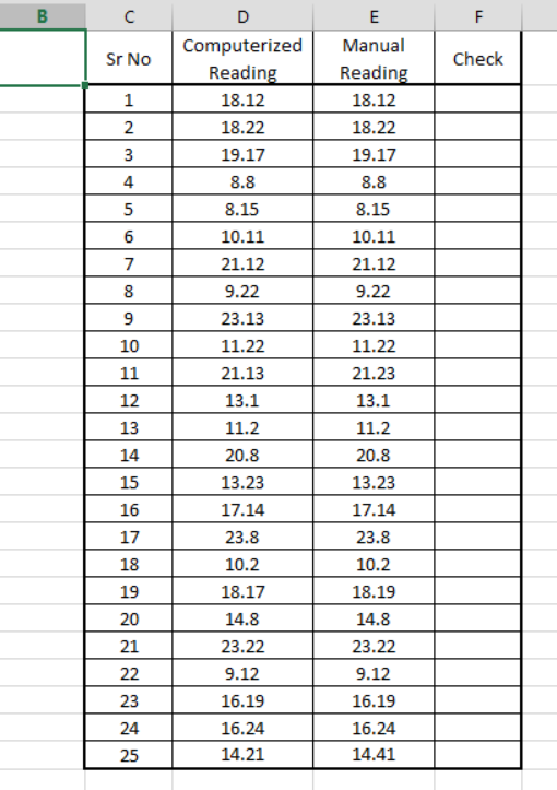Figure 2 – Applying Conditional Formatting

Based on the dataset, we are going to apply conditional formatting.in column F “Check” to see if values in Column D “Computerized Reading” & Column E “Manual Reading” are equal or not.

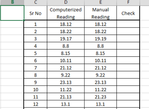Figure 3 – Data

Select cell from “F2:F26” and then click “Conditional Formatting” button from “Home Tab”

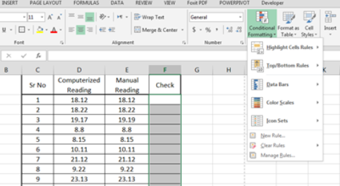Figure 4 – Check Column Selection

Select “New Rule” option from “Conditional Formatting” and by clicking “New Rule” following dialogue box pop up:

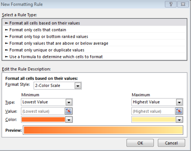Figure 5 – Dialogue Box

In the above mentioned dialogue box, select following “Rule Type” to add formula for conditional formatting, “Use a formula to determine which cells to format”:

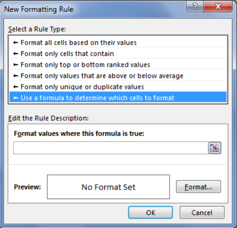Figure 6 – New Formatting Rule

Now we will write formula in the dialogue box:

Formula will be : =D2=E2

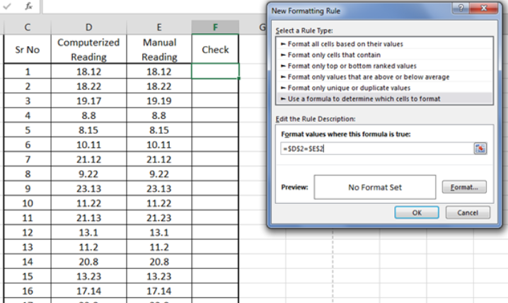Figure 7 – Data & New Formatting Rule Dialogue Box

Now Click button “Format…” to add some formatting if the formula is true and press Ok to close the dialogue box.

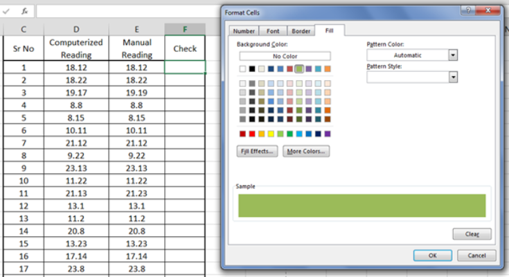Figure 8 – Selection of Color For Conditional Formatting

The formatting is applied for values if they are equal (true). And final result is as follow:

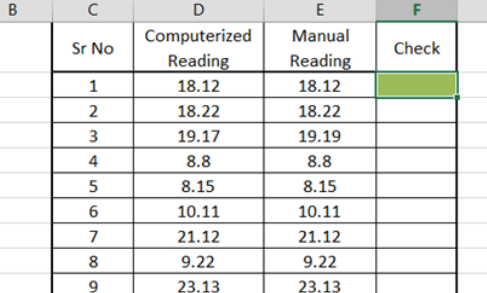Figure 9 – Applying Condition

Now also, we will apply formatting if the formula is not true also in same cell “F2” by following the same steps:

1.    Select cell “F2”
2.    Click conditional formatting from “Home” tab
3.    Select “New Rule”
4.    Select “Rule Type – Use a formula to determine which cells to format”

Formula will be: =D2<>E2

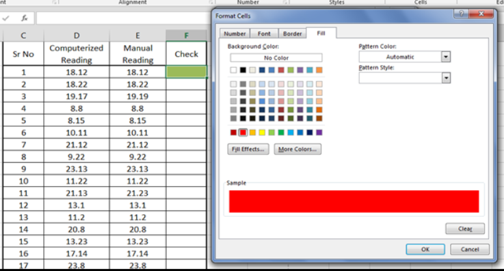Figure 10 – Using Formula Option

5.    Applying formatting by pressing “Format…” and selecting color as you like for value if they are not equal:

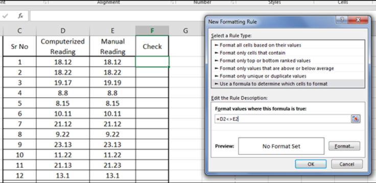Figure 10 – Selection of Color For Conditional Formatting

6.    Press “OK” to close the dialogue box.

Now drag the cell “F2” till the last value and final result be as follow:

Figure 11 – Final Result

We can see in this example  that 4 out of 25 values are not equal to each other i.e., Computerized Reading & Manual Reading and rest of the values are equal.

Most of the time, the problem you will need to solve will be more complex than a simple application of a formula or function. If you want to save hours of research and frustration, try our live Excelchat service! Our Excel Experts are available 24/7 to answer any Excel question you may have. We guarantee a connection within 30 seconds and a customized solution within 20 minutes.