Highlight duplicate values

Excel has some very effective ways to deal with duplicate values. Highlighting duplicates is one such feature. We can easily highlight duplicate values using conditional formatting and the COUNTIF function. In this tutorial, we will learn how to highlight duplicate values in Excel.

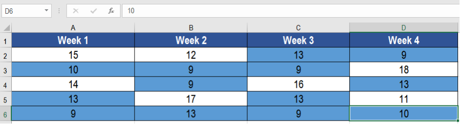Figure 1. Example of How to Highlight Duplicate Values

Generic Formula

=COUNTIF(Range,A1)>1

How the Formula Works

Here, we are using conditional formatting to highlight the duplicate values. The function in use is COUNTIF. The COUNTIF function counts the occurrence of each value in the range. If a value exists more than once, COUNTIF returns TRUE and invokes the formatting rule. .

We use conditional formatting to highlight the cells. Conditional formatting has some preset rules. Still, we are using a custom formula for more flexibility. Excel evaluates the formula used in conditional formatting. It evaluates the formula relative to the cell that is active. This evaluation is done in the selection of the time the rule was created. We are using COUNTIF in the range with an absolute address. But the first cell is relative. Therefore, the range remains unchanged. But, the relative cell A1 changes for each iteration.

Setting Up Data

The following example contains a temperature database during the weekdays of December. Columns A, B, C and D has the name of the winners for each week.

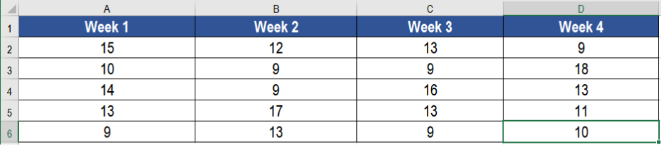Figure 2. The Data Set

To highlight duplicate values, we need to:

• Select cells A2 to D6 with your mouse.
• From the home tab in the ribbon, go to Conditional Formatting > New Rule.

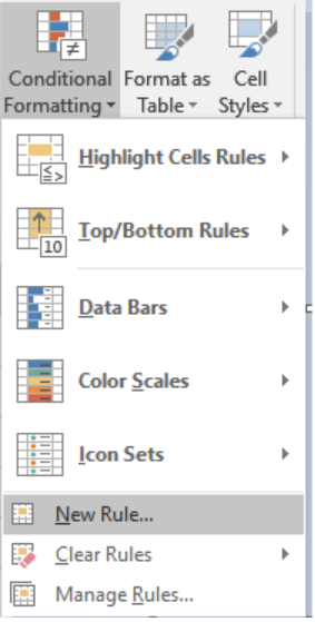Figure 3. Example of how to Apply Conditional Formatting

• Click on Use a formula to determine which cells to format.

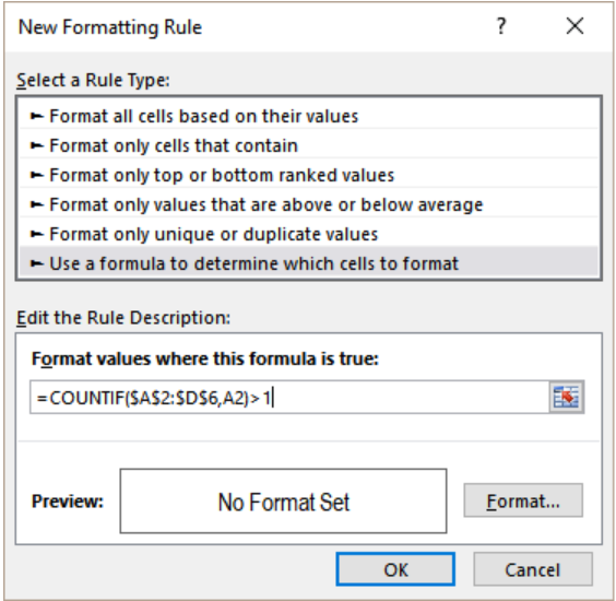Figure 4. Applying the Formula

• In the Format values where this formula is true box, we need to assign the formula =COUNTIF ($A$2:$D$6,A2)>1.  
• Then, we have to click on the Format tab beside the preview box.
• Go to Fill>Background Color and set it to the color you want to highlight to.

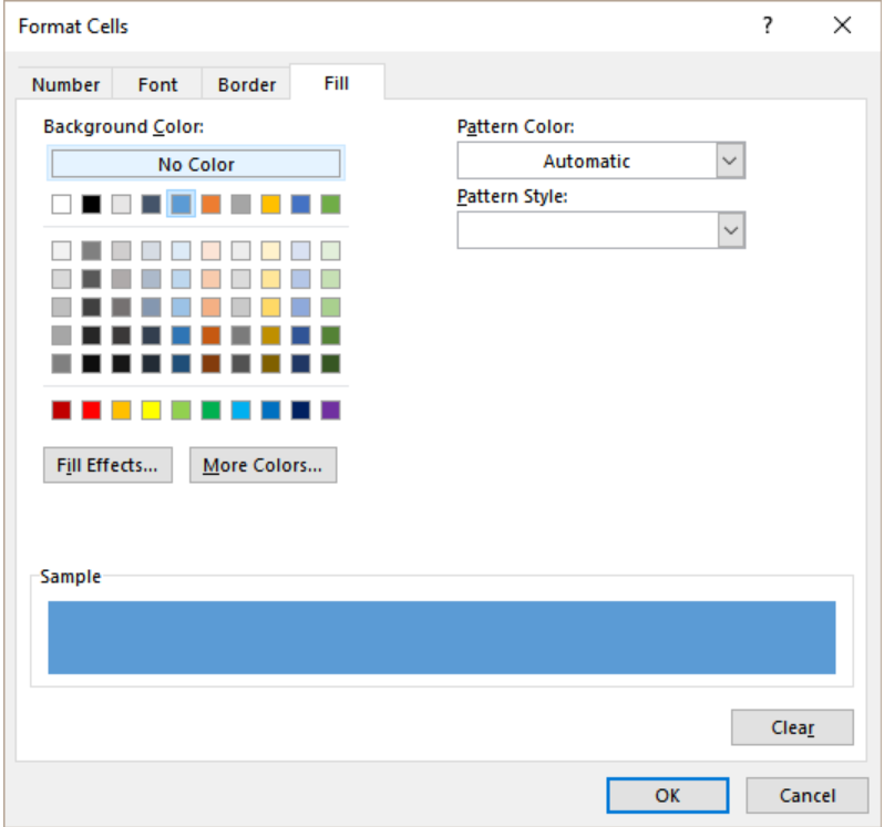Figure 5. Setting the Format of Display

• Click Ok. This will redirect us back to the previous formula box. We need to click Ok for the last time.

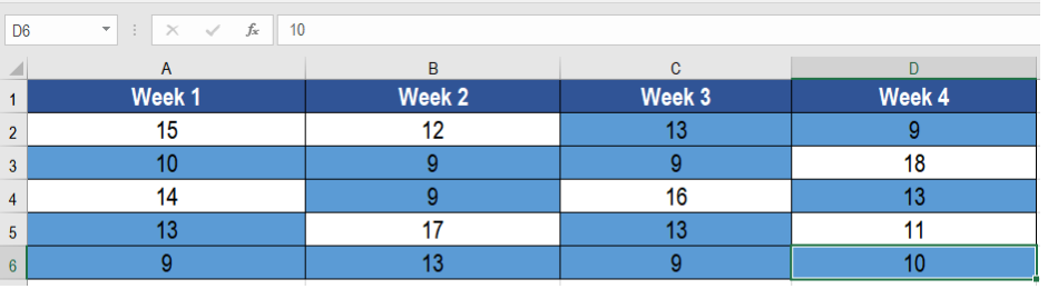Figure 6. Example of the Final Result

This will highlight the duplicate cells containing the temperatures 9,10 and 13 in columns A to D.

Most of the time, the problem you will need to solve will be more complex than a simple application of a formula or function. If you want to save hours of research and frustration, try our live Excelchat service! Our Excel Experts are available 24/7 to answer any Excel question you may have. We guarantee a connection within 30 seconds and a customized solution within 20 minutes.