How to Highlight Duplicate Columns in Excel using a Formula

Working on a large database can often create confusions. It is not uncommon to create duplicate columns by mistake. Excel offers a great fix to diagnose if there are identical columns. We can do this by highlighting duplicate columns. We use the SUMPRODUCT function along with conditional formatting to do this. In this lesson, we will learn how to highlight duplicate columns in Excel.

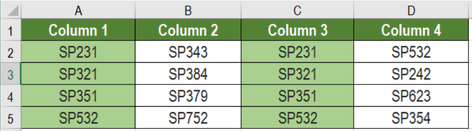Figure 1. Example of How to Highlight Duplicate Columns in Excel

Formula

=SUMPRODUCT ((row1=reference1) * (row2=reference) * (row3=reference3)) >1

This formula is based on the SUMPRODUCT function. It counts how many times each value occurs in the table, in a row wise manner. The function will provide TRUE if the values are same in all the rows.

We use absolute row references. But the cell references are mixed, where the row is locked. This checks all instances of the row for duplicates.

Setting up Data

The following database contains some sample text. Column A to D has these texts.

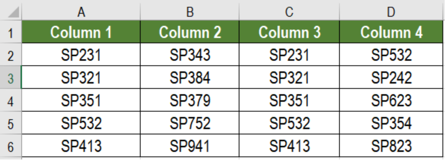Figure 2. The Data Set

To highlight duplicate columns, we need to:

• Click on cell A2. Drag the selection from cells A2 to D6.
• In the home tab of the ribbon, click Conditional Formatting > New Rule.

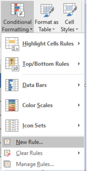Figure 3. Example of how to Apply Conditional Formatting

• Select Use a formula to determine which cells to format.

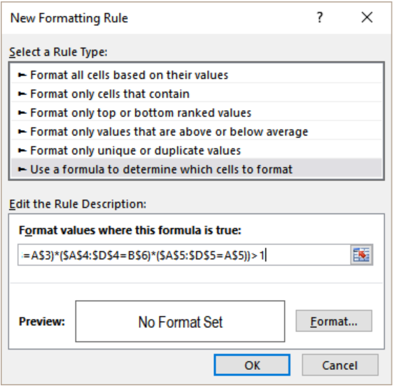Figure 4. Applying the Formula

• Next, we need to assign the formula =SUMPRODUCT(($A$2:$D$2=A$2)*($A$3:$D$3=A$3)*($A$4:$D$4=A$4)*($A$5:$D$5=A$5))>1. This needs to be assigned in the Format values where this formula is true box,
• Next, we need to click on Format.
• Select Fill>Background Color and set it to the color of your choice.

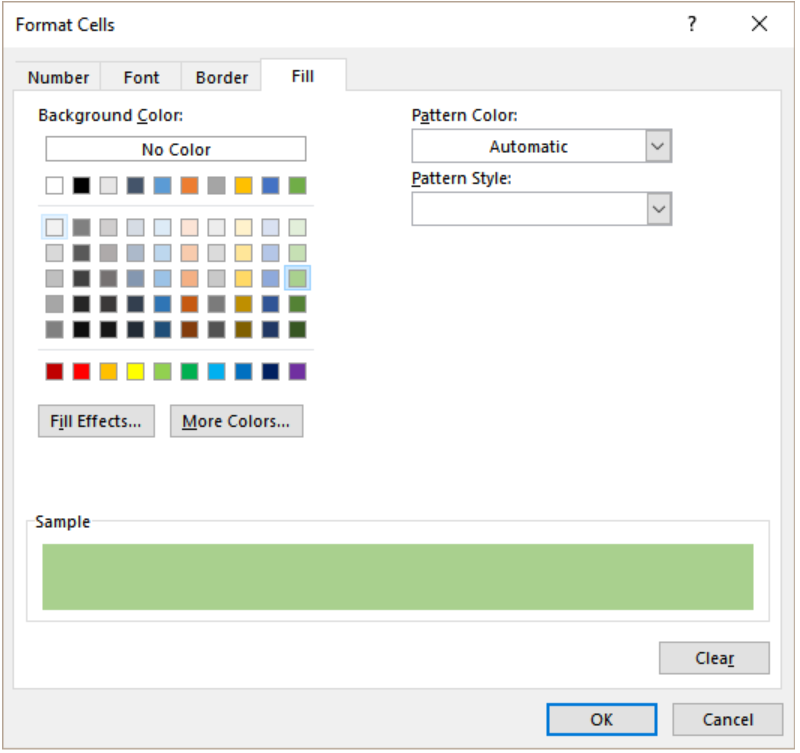Figure 5. Formatting the Display

• Click Ok twice.

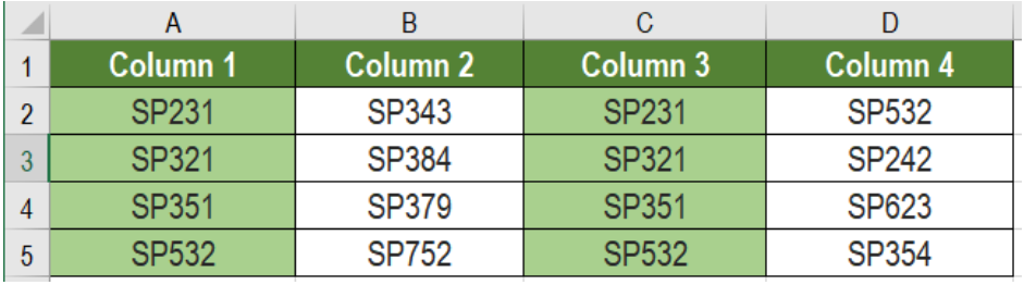Figure 6. The Final Result

This will highlight the duplicate columns B and C using the conditional formatting.

Most of the time, the problem you will need to solve will be more complex than a simple application of a formula or function. If you want to save hours of research and frustration, try our live Excelchat service! Our Excel Experts are available 24/7 to answer any Excel question you may have. We guarantee a connection within 30 seconds and a customized solution within 20 minutes.