

Conditional Formatting is an excellent way to visualize the data based on certain criteria. OR function in the Conditional Formatting highlights the data in the table if at least one of the defined conditions is met. This step by step tutorial will assist all levels of Excel users in creating a Conditional Formatting OR formula rule.
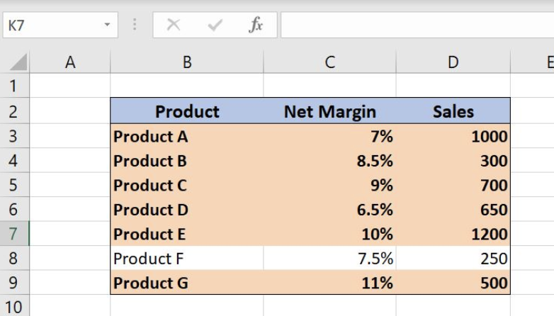
Figure 1. Final result
Syntax of the OR formula
=OR(logical1,[logical2], …)
The parameters of the OR function are:
- Logical1, logical2 – the conditions that we want to test
The output of the formula is value TRUE if just one condition is met. If neither of the conditions is met formula result will be FALSE
Highlight cell values using OR function
To mark the rows in the table based on the certain criteria we can use formula rules in the Conditional Formatting. In our example, we want to emphasize the rows in the table where Net Margin is over 8% or Sales are over 600. For this purpose, we will use OR function since it’s enough that only one condition is met.
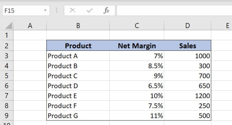 Figure 2. Highlight rows where Net Margin is over 8% or Sales is over 600
Create an OR formula rule in the Conditional Formatting
To create a Conditional Formatting rule based on the formula we should follow the steps below:
- Select the cell, cell range or table in Excel where we what to apply the Conditional Formatting
 Figure 3. Select a cell range for the Conditional Formatting
- Find Conditional Formatting button tab and choose New Rule
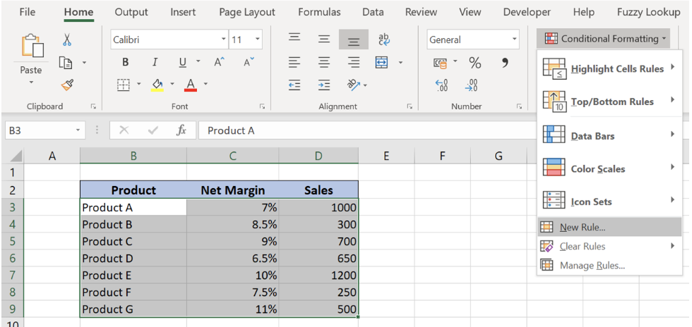 Figure 4. Create a new rule in the Conditional Formatting
- Choose Use a formula to determine which cells to format
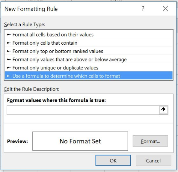 Figure 5. Create a formula rule in Conditional Formatting
- Enter formula rule under the section Format values where this formula is true
=OR($C3>8%,$D3>600)
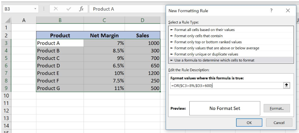 Figure 6. OR function in Conditional Formatting
The formula above highlights the rows in the example table where Net Margin is over 8% or Sales is over 600. OR function checks if at least one condition is met and returns the value TRUE. This value triggers the Conditional Formatting rule.
In our OR formula example there are two logical tests:
- Logical1 is $C3>8% – checks if Net Margin is over 8%
- Logical2 is $D3>600 – examines if Sales is over 600
- Under the Format tab, we can define the visual appearance of the cells if the OR formula output is TRUE
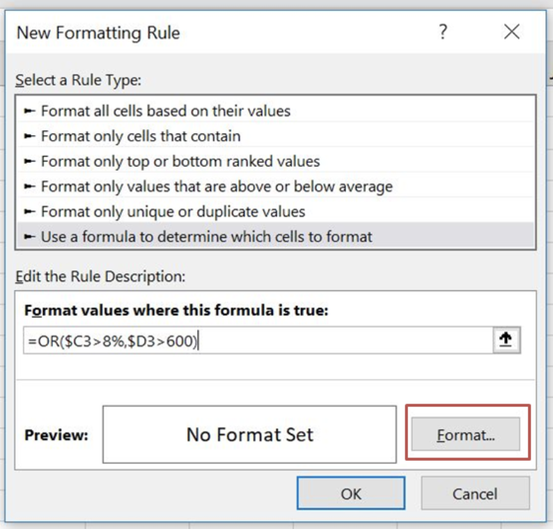 Figure 7. Create a custom format in Conditional Formatting
- In Fill tab choose the background color (here you can also choose pattern style and color)
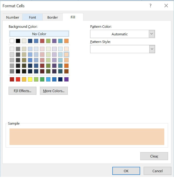 Figure 8. Define a Background Color of the cells
- In the Font tab we can define font style and Bold cell text
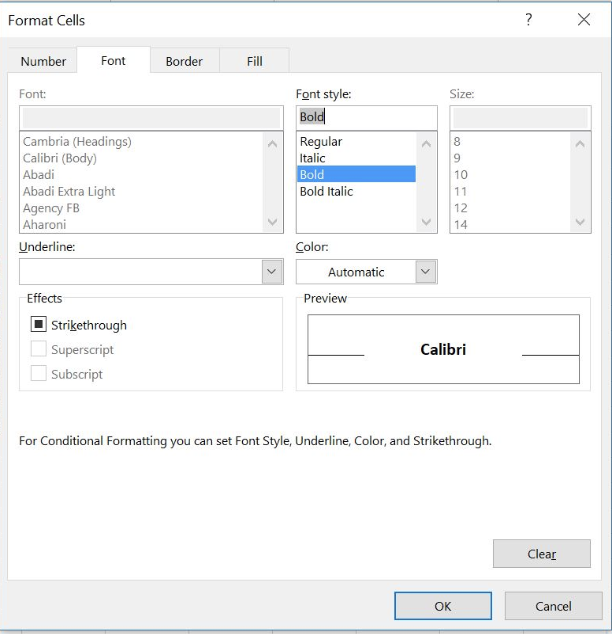 Figure 9. Choose a Font style of the cells
- After choosing the format in section Preview we can see how Conditional Formatting cells will look like if the rule is met
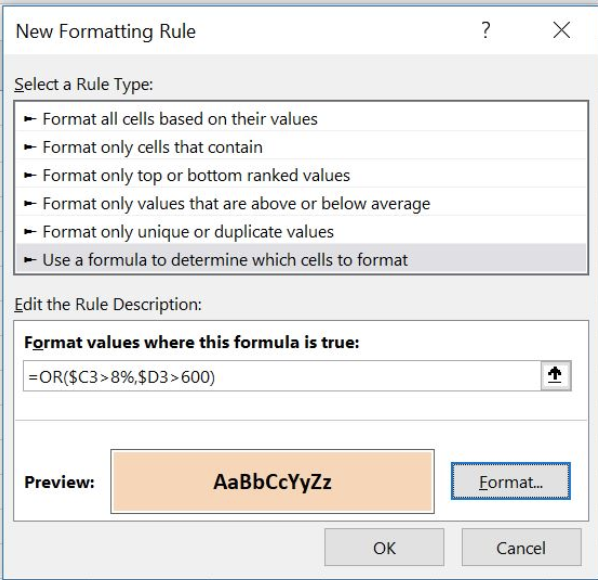 Figure 10. Conditional Formatting rule Preview
- Rows in the table are highlighted whenever the Net Margin is over 8% or Sales is over 600. Product F in the table is the only product that meets neither Net Margin nor Sales condition.
Figure 11. Conditional Formatting OR formula rule- Net Margin over 8% or Sales over 600
Most of the time, the problem you will need to solve will be more complex than a simple application of a formula or function. If you want to save hours of research and frustration, try our live Excelchat service! Our Excel Experts are available 24/7 to answer any Excel question you may have. We guarantee a connection within 30 seconds and a customized solution within 20 minutes.


Leave a Comment