Here’s How You Can Use Conditional Formatting If Two Cells Are Not Equal

Conditional formatting is one of the most useful functions of Excel. This step by step tutorial will assist all levels of Excel users in conditional formatting two cells that are not equal.

Example 1

Figure 1. Setting the data

This data refers to the total and obtained GPA of students. Only those students will be selected for scholarship that got 4 out of 4 GPA.

We need to use conditional formatting to highlight the students with a GPA less than 4 in order to avoid them for selection.

Or we can say, we need to highlight the cells of Column C and F that are not equal to the cells of Column B and E.

Steps

• Select cells of column C from C2 to C14.

• Select conditional formatting in the “Styles” section of the toolbar.

• Click the option of “New Rule” and “New formatting Rule” window will appear.

• Choose the rule type written as “Use a formula to determine which cells to format” from window.

• In order to write the formula in the “Rule Description” bar, Select cell C2 to C14, put a “Not Equal to” sign and then select cells from B2 to B14.

(The sign <> is referred as “Not Equal to” sign in Excel)

• Now click on the ‘format” option to select format of your choice like color of the formatted cells etc.

Figure 2. Applying formatting rule for example 1

“New Formatting Rule” window will appear like this. Press OK to apply conditional formatting.

Do the same with Column F and the unequal cells will appear highlighted as given in the figure below.

Figure 3. Result of example 1

Example 2

Figure 4. Applying formatting rule for example 2

This is another example of conditional formatting where cells are not equal.

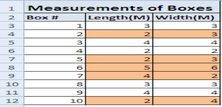
In this example, we’ll apply conditional formatting in order to highlight the boxes with unequal length and width.

We can separate unequal boxes from the boxes of equal measurements with the help of conditional formatting.

Same process and formula from Example # 1 is followed in Example # 2 and the final figure is given below.

Figure 5. Result of example 2

Note

The formula is automatically locked in the rule description section and appears like this:

Figure 6. Formula

Remove the $ sign before the number of rows/numerical figures to get accurate results.

Most of the time, the problem you will need to solve will be more complex than a simple application of a formula or function. If you want to save hours of research and frustration, try our live Excelchat service! Our Excel Experts are available 24/7 to answer any Excel question you may have. We guarantee a connection within 30 seconds and a customized solution within 20 minutes.