How to Use Conditional Formatting Dates in Excel

Conditional formatting in Excel can be used to format dates based on whether certain criteria are met. We can use a variety of formatting options, including color.

Setting up the Data

In the example below, if a particular date is past 60 days from the current date, we will color the cell orange.

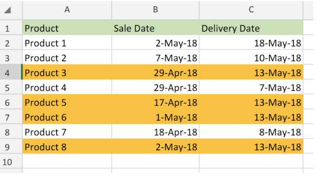Figure 1. Conditional Formatting of Dates in Excel.

Application of Conditional Formatting Rules in Excel

This can be done in 5 simple steps.

1. Select the range of dates for formatting.

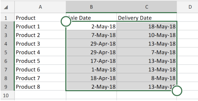Figure 2. Highlighted range of dates in Excel.

2. Open the “Conditional Formatting” drop down tab from the “Styles” group located on the “Home” tab.

Figure 3. Conditional Formatting tab in Excel.

3. From the “Highlight Cells Rules” fly out, click on one of the date options, such as “A Date Occurring”..

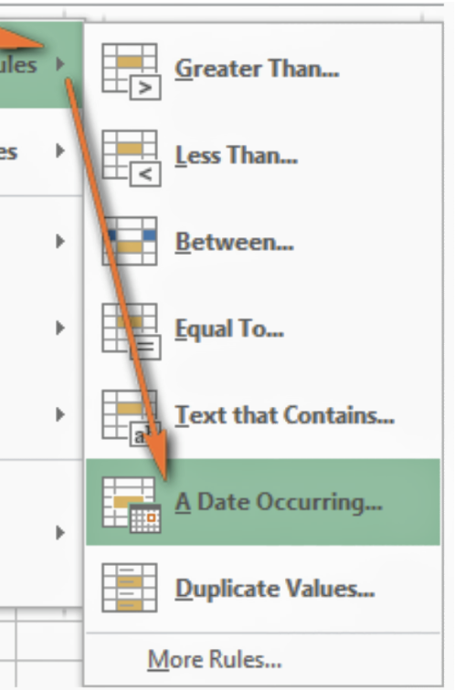Figure 4. Highlight Cell Rules in Excel.

4. This will enable us to specify the criteria we need. In this example, we would like to apply Conditional Formatting (orange color) to the last 7 days of our example. Note that the current date we are working with is the 18th of May 2018.

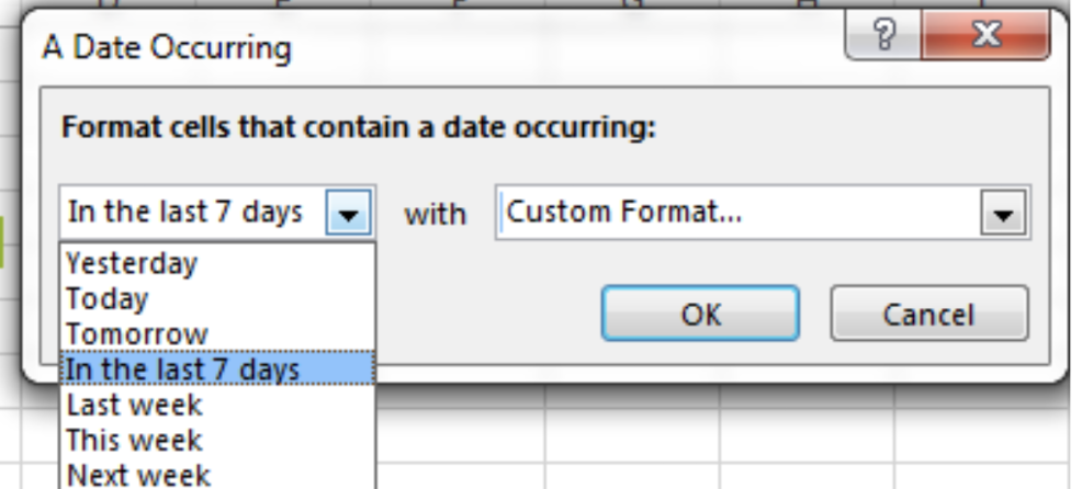Figure 5. of A Date Occurring specification in Excel.

4. We can select one of the inbuilt formats or customize our own date format by choosing from the different available options located on the “Border”, “Font” and “Fill” tabs. If the standard Excel color palette is not sufficient for us, we have the ”More Colors” button available.

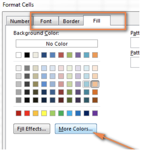Figure 6. of Format Cells in Excel.

5. Click on “ok” and view the result.

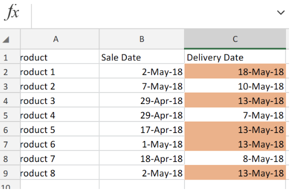Figure 7. of Conditional Formatting of Dates in Excel.

Note however, this quick and straightforward method has two(2) important limitations.

1. Application of Conditional Formatting is always based on the current date/day. Excel has provided us with the “Today” Function for calculations based on the current date. These can be used to conditionally format dates entered into our Excel sheet. To use the Today Function to conditionally format cells based on today’s date, input the any of the “Today Operation Syntax” provided below, in the formula bar of our Conditional Formatting Rules Manager. We can find the Rules Manager on our current worksheet by clicking on the “Home” tab, within the “Styles Group” click on the “Conditional Formatting” icon. Click on the “Manage Rules” icon, the “Conditional Formatting Rules Manager” icon appears.

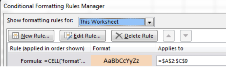Figure 8. of Conditional Formatting Rules Manager in Excel.

Note that because we are going to select cell A1 Excel will by default apply our rules to the cell range A1 to A9.

Today Operation Syntax

• Equal to today =$B2=TODAY()
• Less than today =$B2<TODAY ()
• Greater than today =$B2>TODAY ()

The image below provides a demonstration of the rules above. Kindly note that the current date of writing for our example is the date in cell B2, 2nd  of May 2018:

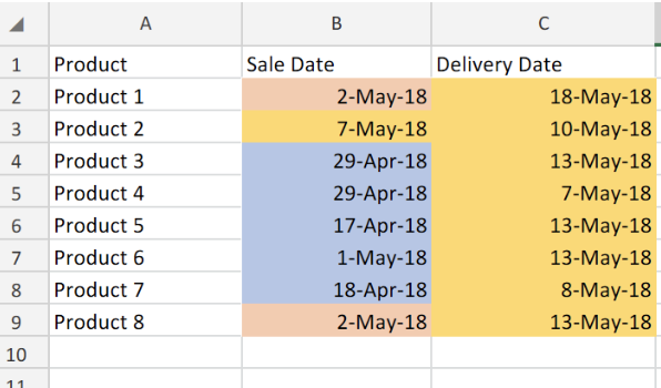Figure 9. of the application of Today Function for Conditional Formatting in Excel.

2. It works on highlighted cells only.

For dates, Excel’s conditional formatting options simplify the process of differentiating between weekends and weekdays, displaying an approaching deadline day, or highlighting scheduled delivery dates on our worksheet.

In this post, we have illustrated how to apply conditional formatting to dates in our Excel worksheet, based on whether they meet certain criteria.

Instant Connection to an Expert through our Excelchat Service:

Our live Excelchat Service is here for you. We have Excel Experts available 24/7 to answer any Excel questions you may have. Guaranteed connection within 30 seconds and a customized solution for you within 20 minutes.