

Conditional Formatting is an excellent way to visualize the data based on certain criteria. This step by step tutorial will assist all levels of Excel users in creating a Conditional Formatting and applying it across multiple cells.
Setting up Our Data for Conditional Formatting
Our table consists of 3 columns: “Month” (column B), “Salesman ” (column C) and “Sales” (column D). We want to highlight cells in column D if the value in the cell is greater than $500.
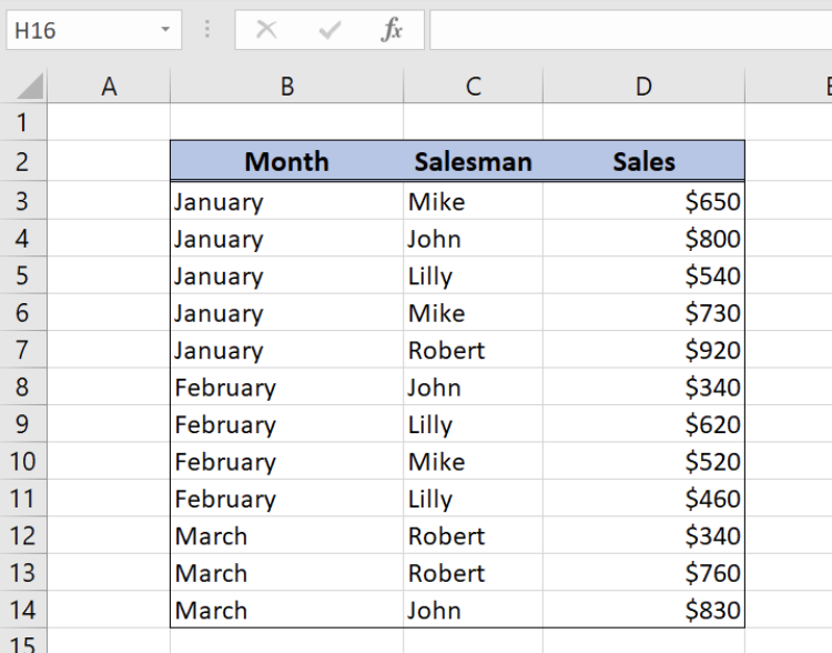 Figure 1. Data for Conditional Formatting
Highlight cell values based on a condition
To mark the cell in column D based on the certain criteria we can use formula rules in the Conditional Formatting. First, we will create a rule for the cell D3. To create a Conditional Formatting rule we should follow the steps below:
- Select the cell, where we what to apply the Conditional Formatting – in our case D3. Find Conditional Formatting button tab and choose New Rule:
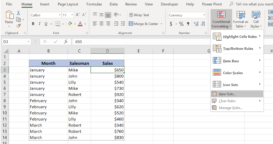 Figure 2. Create a new rule in the Conditional Formatting
- Choose Format only cells that contain and then choose cell value greater and enter 500:
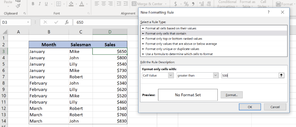 Figure 3. Choose a Rule Type
- Now click on the Format button, where we can define the visual appearance of the cell:
- In Fill tab, choose the background color (here you can also choose pattern style and color)
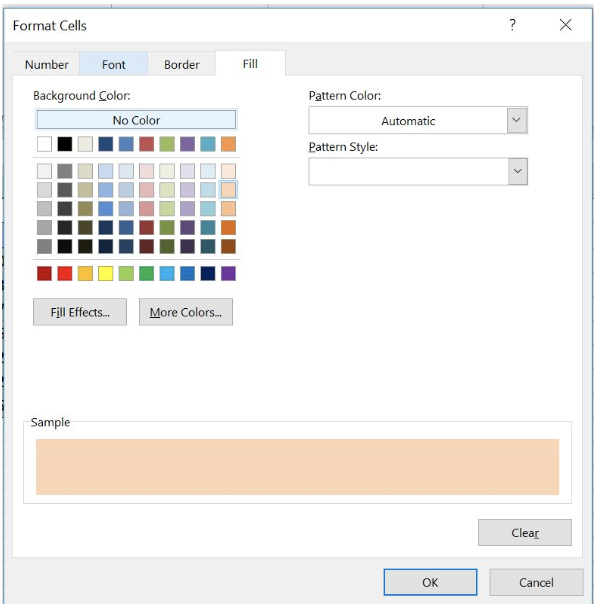 Figure 4. Define a Background Colour of the cells
- In the Font tab, we can define font style and Bold cell text:
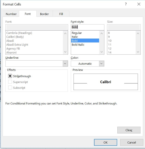 Figure 5. Choose a Font style of the cells
- After choosing the format in section Preview we can see how Conditional Formatting cell will look like if the rule is met:
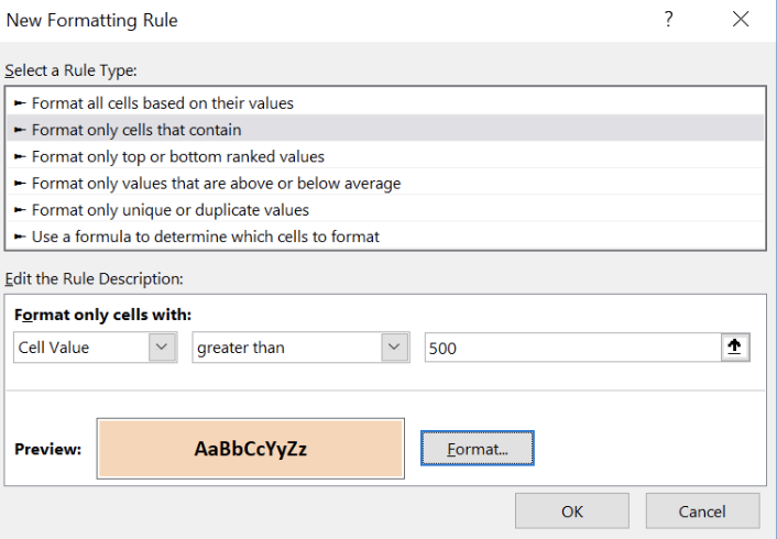 Figure 6. Conditional Formatting rule Preview
- Cell D3 has value $650, which is greater than $500, so our conditional formatting is applied to the cell:
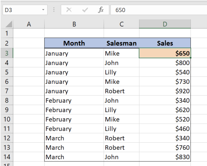 Figure 7. Conditional formatting of the cell D3
Using Conditional Formatting Across Multiple Cells
Now we want to apply our conditional formatting from the cell D3 to all Sales (range D4:D14). To do this, we will use the format painter. Here are the steps:
- Select the cell with conditional formatting – D3
- Click on the format painter icon in the Home tab:
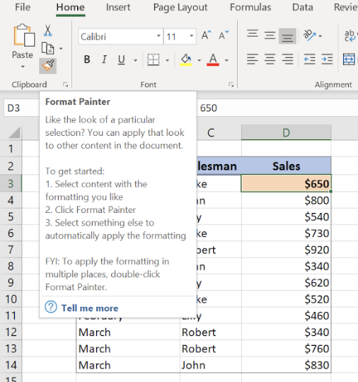 Figure 8. Use format painter
- Select the range where we want to apply conditional formatting – D4:D14:
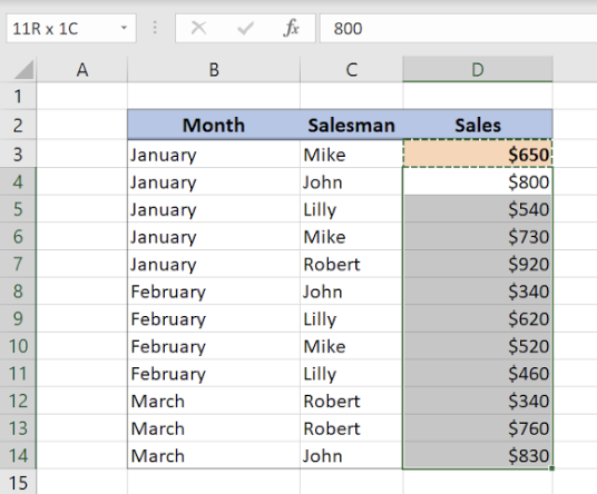 Figure 9. Use format painter
Now we have our conditional formatting successfully applied to all cells in the range D3:D14. We can see, all the values greater than $500 are highlighted.
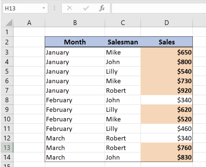 Figure 10. Conditional formatting applied to multiple cells
Most of the time, the problem you will need to solve will be more complex than a simple application of a formula or function. If you want to save hours of research and frustration, try our live Excelchat service! Our Excel Experts are available 24/7 to answer any Excel question you may have. We guarantee a connection within 30 seconds and a customized solution within 20 minutes.


Leave a Comment