

To make Excel gauge chart we combine Excel Doughnut and Pie charts in a single chart, which is also known as Excel speedometer or Dial chart because we visualize the information as a reading on a dial. The Doughnut chart is used to show the contribution of each value to a total as a colored data range and the Pie chart is used as a pointer related to that colored data range.
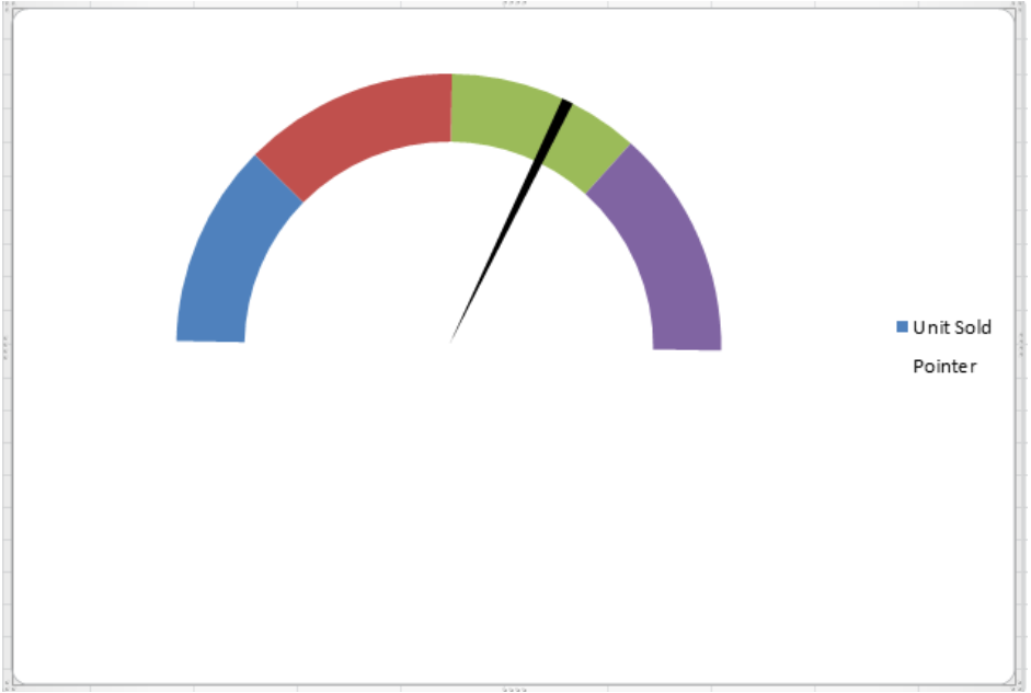 Figure 1. Gauge Chart
How to Make Gauge Chart
Suppose we have data from different regions for their units sold against a target to meet. We want to show the information on Gauge chart of the contribution of each region to a total number of unit sold against a set target to achieve.
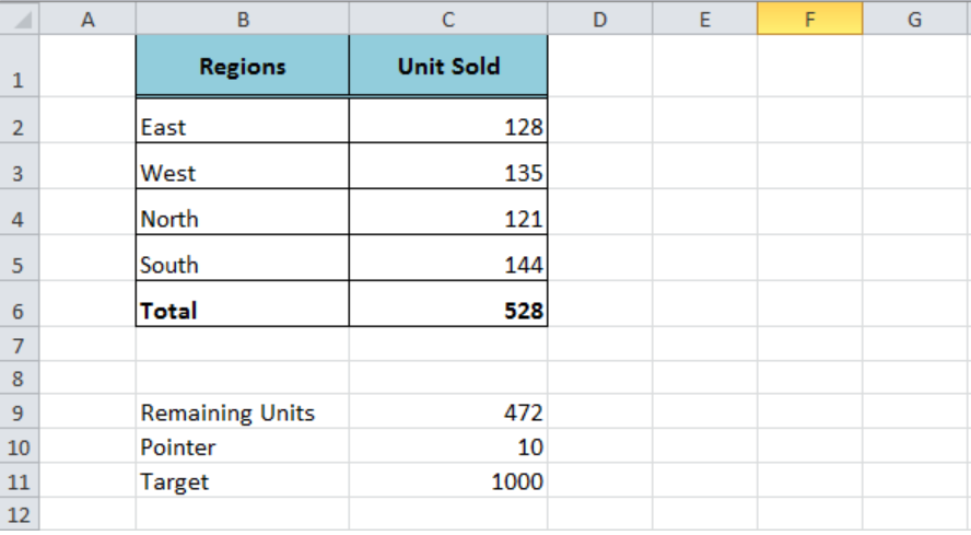 Figure 2. Data Set
To make Gauge chart we need to follow these steps;
- First, we need to make a Doughnut chart for units sold in each region. Select the data range B2: C6 in our example.
- Go to Insert tab, Click on Other Charts and select Doughnut
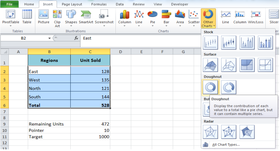 Figure 3. Insert Doughnut Chart
- Right-click inside the chart markers and select Format Data Series option
 Figure 4. Format Data Series of Doughnut Chart
- In Series Options, enter the Angle of the first slice as 271 and increase the Doughnut Hole size to 75%.
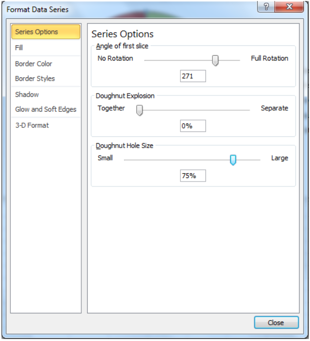 Figure 5. Formatting Data Series
- Select the Total data point and right-click to select the Format Data Point
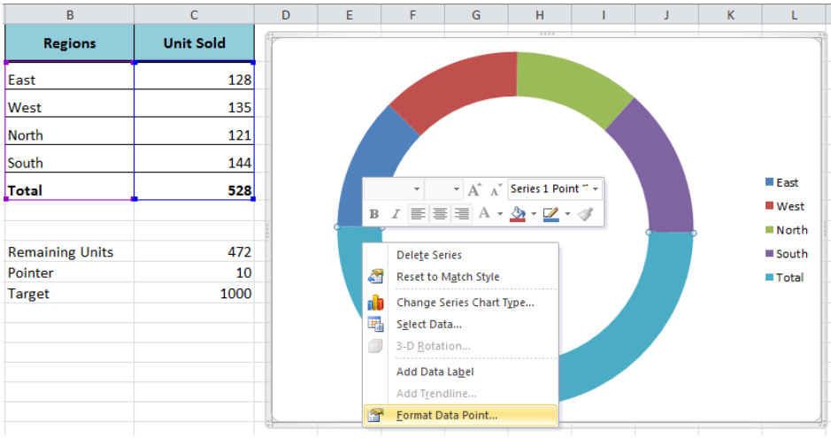 Figure 6. Formatting Data Point
- Click on the Fill menu and select No Fill to disappear the Total data point.
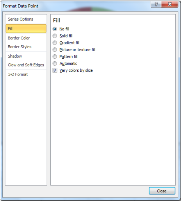 Figure 7. Select No Fill
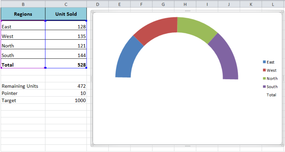 Figure 8. Doughnut Chart
- To create Pie chart inside this chart, right-click inside the chart area and click on Select Data
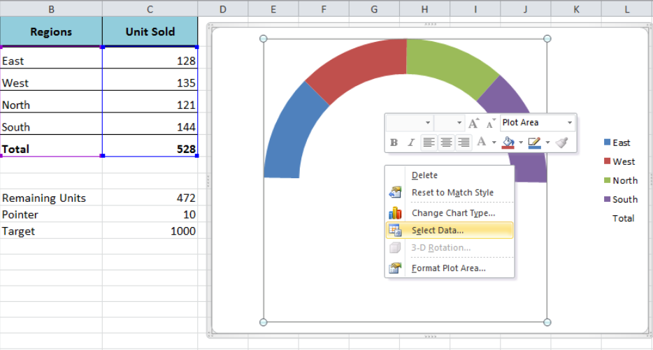 Figure 9. Clicking Select Data Option
- Click on Add button to insert the second series data for Pie chart.
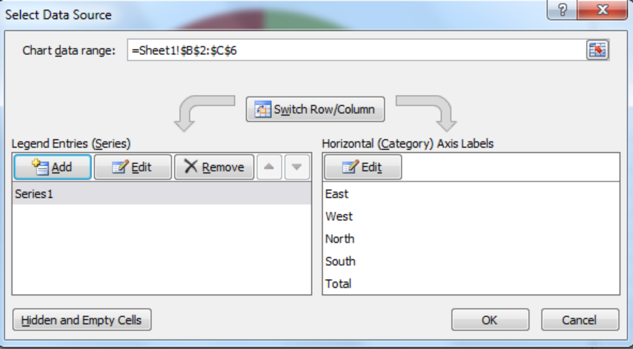 Figure 10. Adding Data Series for Pie Chart
- Enter the Series Name as “Pointer” and select the data range C9: C11 in our example.
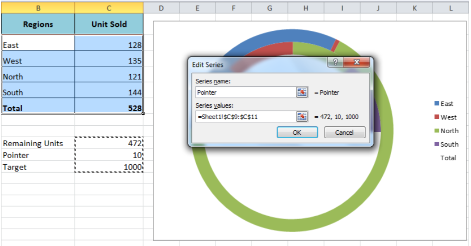 Figure 11. Entering Data Range For Pie Chart
- By default, Excel creates another Doughnut chart, we have to change its type.
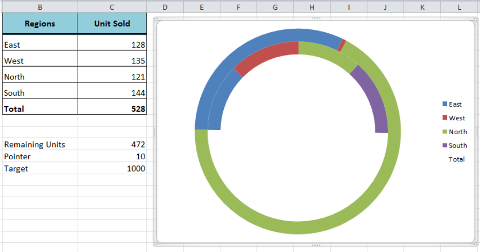 Figure 12. Doughnut Chart For Series 2
- Select the outer Doughnut chart and right-click to select Change Series Chart Type option
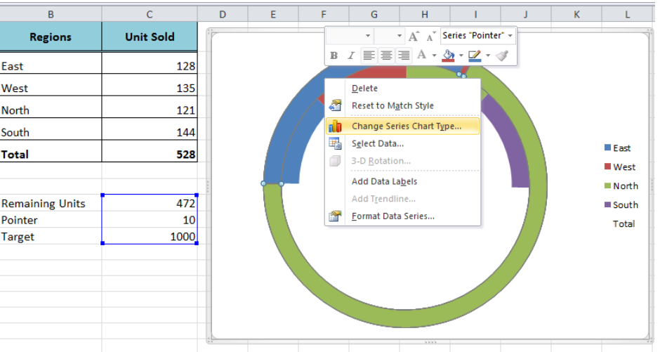 Figure 13. Changing Chart Type
- Select the Pie chart and press the OK button.
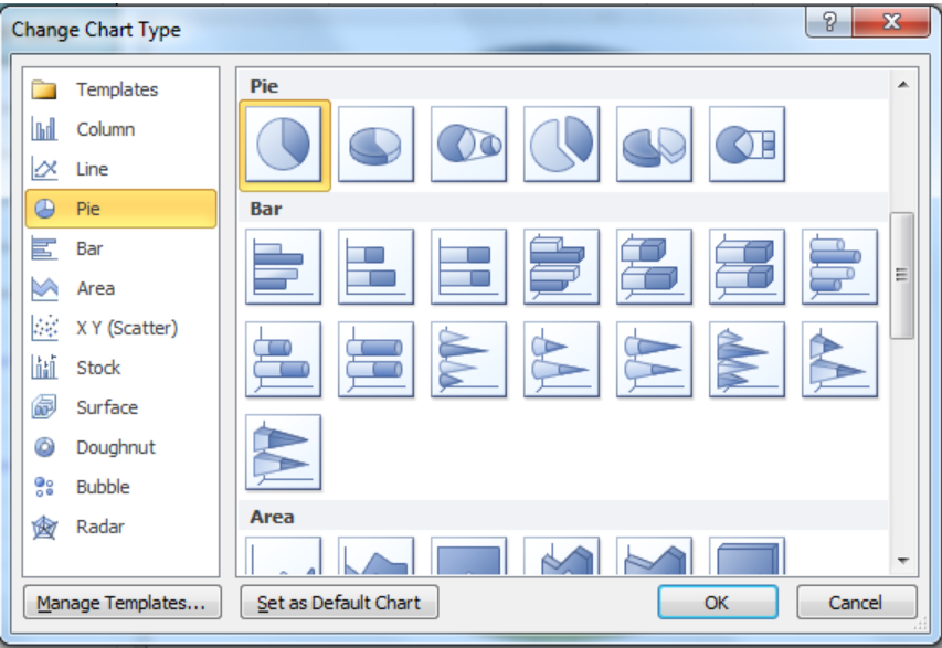 Figure 14. Selecting Pie Chart Type.
- Right-click inside the Pie chart and select Format Data Series option.
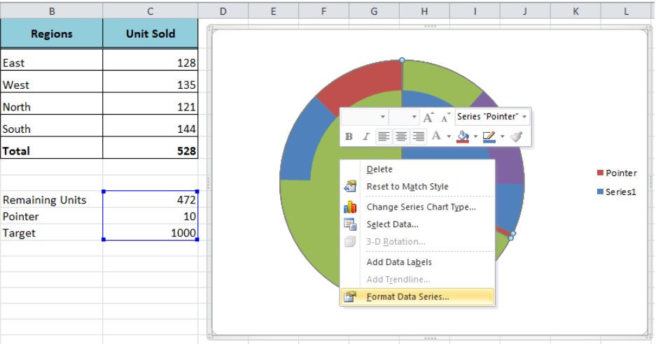 Figure 15. Format Data Series of Pie Chart
- Enter the Angle of the first slice as 270 and select plot series on the Secondary axis.
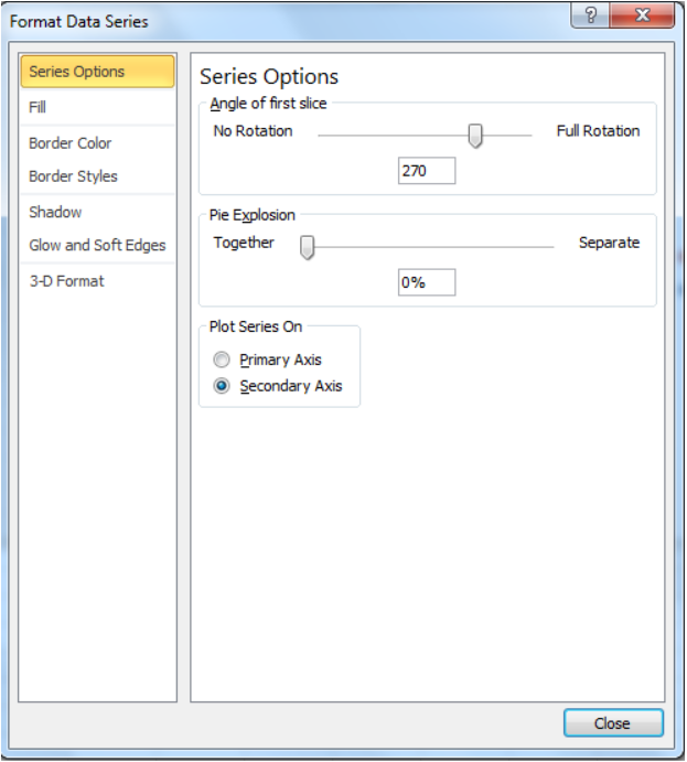 Figure 16. Formatting Data Series of Pie Chart.
- Now select the large slices of Pie chart, one by one, right-click > Select Format Data Point and select Fill > No Fill.
 Figure 17. Formatting Data Points Of Pie Chart
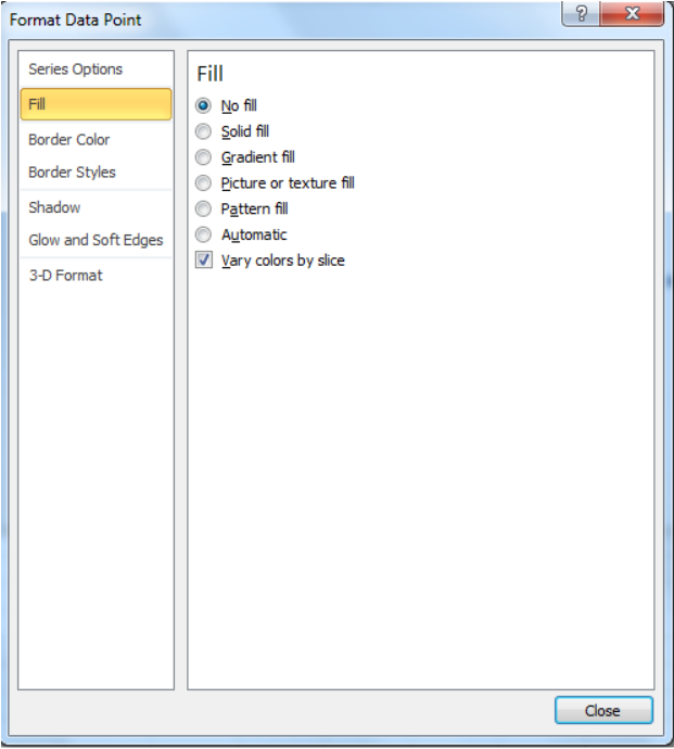 Figure 18. Selecting No Fill For Data Point
- After formatting the large slices of Pie Chart as No Fill, only the small data point of Pie chart remains visible to show as meter Pointer that is the final view of the Gauge chart.
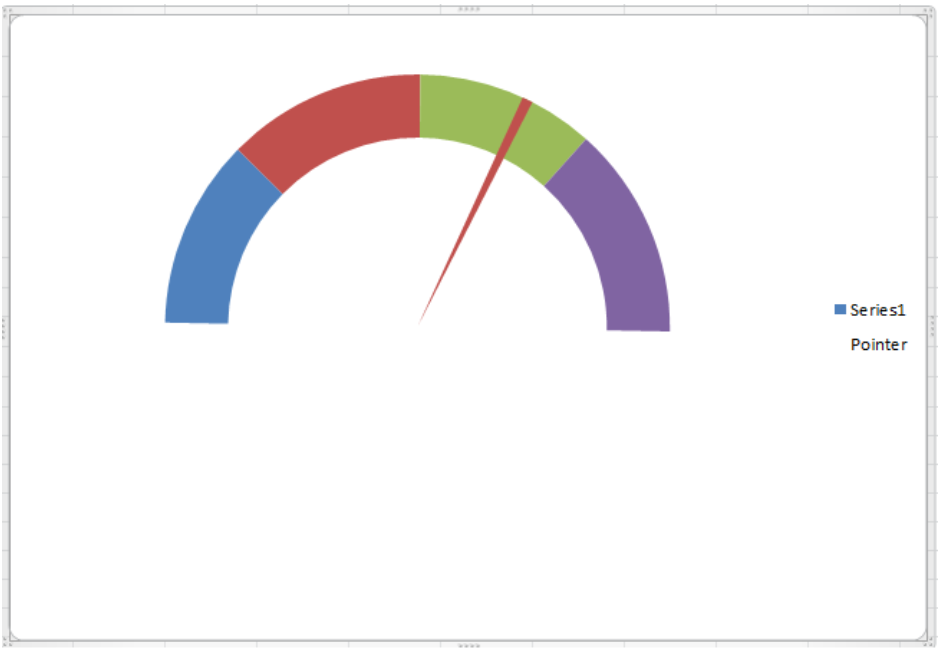 Figure 19. Gauge Charts
Instant Connection to an Expert through our Excelchat Service
Most of the time, the problem you will need to solve will be more complex than a simple application of a formula or function. If you want to save hours of research and frustration, try our live Excelchat service! Our Excel Experts are available 24/7 to answer any Excel question you may have. We guarantee a connection within 30 seconds and a customized solution within 20 minutes.


Leave a Comment