

We can change our chart style in Microsoft excel by using the predefined chart styles in the design menu on our taskbar. The design menu automatically appears immediately we select a chart. This tutorial will teach us how to change our chart style.
 Figure 1: Changing chart style
Data to change chart style in Excel 2016
- We will prepare a table to create our chart
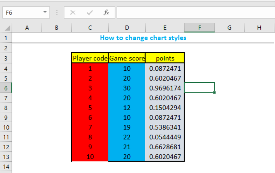 Figure 2: Data to change chart style in excel 2016
- We will create our chart by highlighting the table, then we will select insert in the menu section. We will select any chart type we want by click on the various shapes of chart displayed as icons in the Charts group. We can also use the recommended charts option, if we do not have an ideal chart in mind.
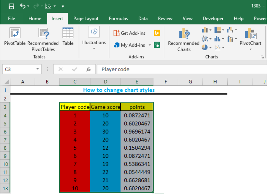 Figure 3: Selecting the chart option
- After selecting our chart, the chart will then be displayed on the page.
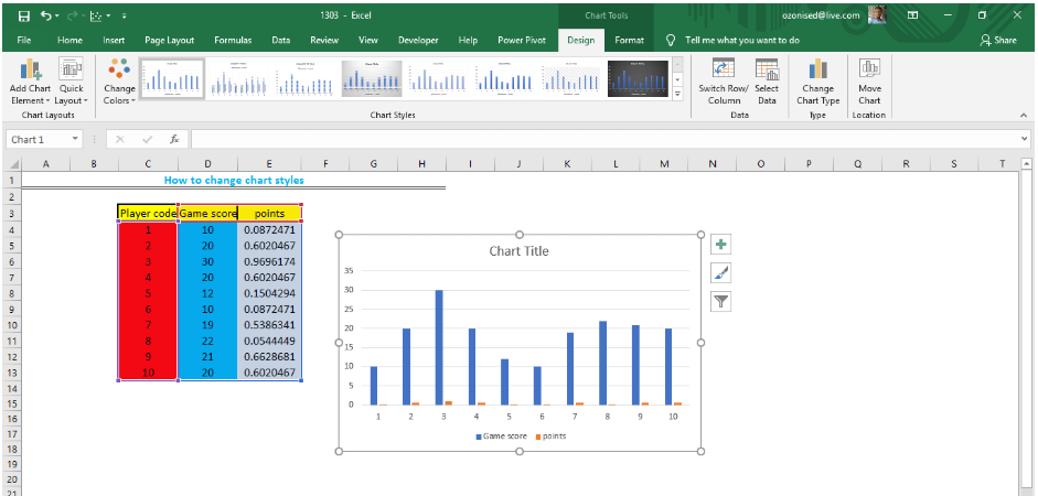 Figure 4: Selected chart
- With the chart still highlighted, we will use the Design option displayed automatically above our page on the task bar to change the style of our chart. We can also use the quick layout to change the style of our chart.
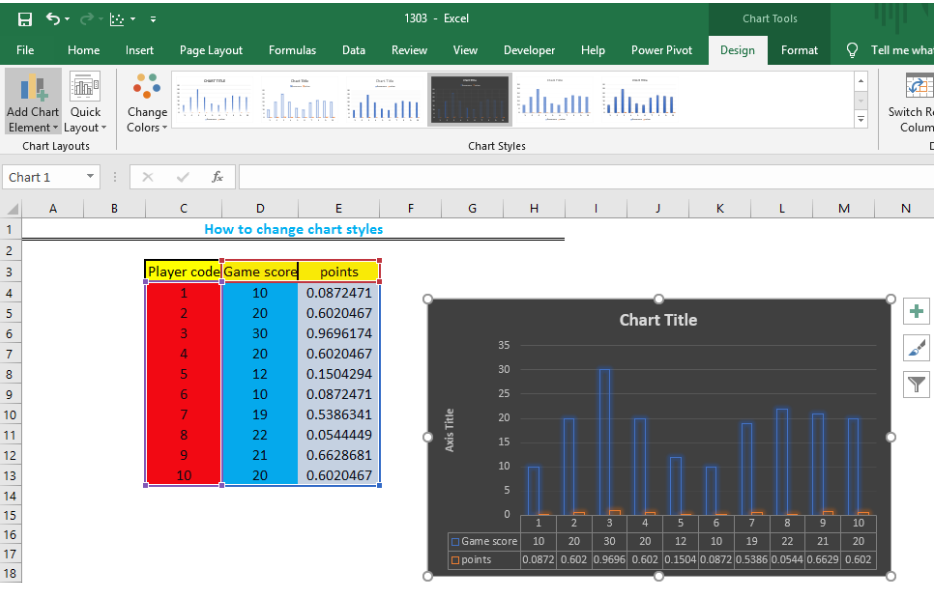 Figure 5: Edited Chart style
Instant Connection to an Expert through our Excelchat Service
Most of the time, the problem you will need to solve will be more complex than a simple application of a formula or function. If you want to save hours of research and frustration, try our live Excelchat service! Our Excel Experts are available 24/7 to answer any Excel question you may have. We guarantee a connection within 30 seconds and a customized solution within 20 minutes.


Leave a Comment