

We can use a formula that combines the MEDIAN and IF functions to find the median of a set of data if the values meet a criteria in a Pivot Table. The steps below will walk through the process.
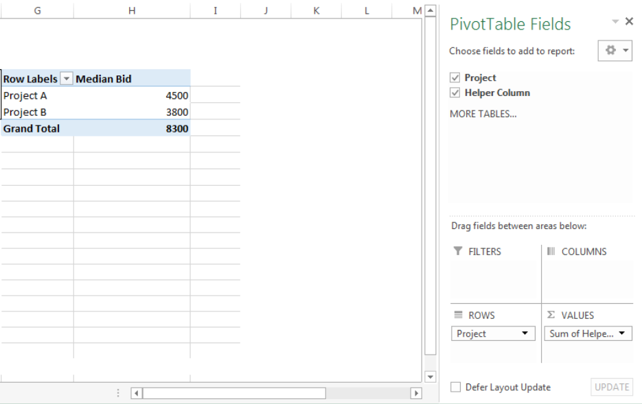
Figure 1- How to Find the Median in a Pivot Table
Syntax
=MEDIAN(IF(logical_test,value_if_true,value_if_false))
- logical_test: This is the criteria that must be met for the median function to operate
- value_if_true: This is the returned result by the IF Function that tells the median function that the criteria is met and the median function can operate
- value_if_false: This is the opposite of value_if_true
Formula
=MEDIAN(IF($B$5:$B$10=E5,$C$5:$C$10))
Setting up the Data
Contractors have placed their bids for two separate projects in a company. The manager intends to find the median bid for Project A and Project B with a Pivot Table
- We will insert the Project names and Bids in Column B and Column C respectively
- Pivot Tables do possess the MEDIAN Function, hence, we have created a helper column in Column F
 Figure 2 – Setting up the Data
How to Create the Helper Column
- We will click on Cell F5
- We will insert the formula below into Cell F5
=MEDIAN(IF($B$5:$B$10=$E$5,$C$5:$C$10)) - Because this is an array formula, we will press CTRL + SHIFT + ENTER
- We will click on Cell F5 again
- We will double click on the fill handle tool which is the small plus sign you see at the bottom right of Cell F5. Select and drag down to copy the formula to Cell F6.
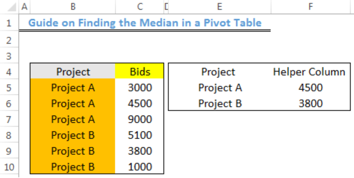 Figure 3- Creating the MEDIANIF Helper Column
Creating the Pivot Table
- We will select the range (E4:F6) of the table containing the helper column
- We will click on Cell G4 where our PIVOT TABLE will be returned in the existing worksheet
- We will click on the Insert tab and click on Pivot Table
 Figure 4- Clicking on Pivot Table
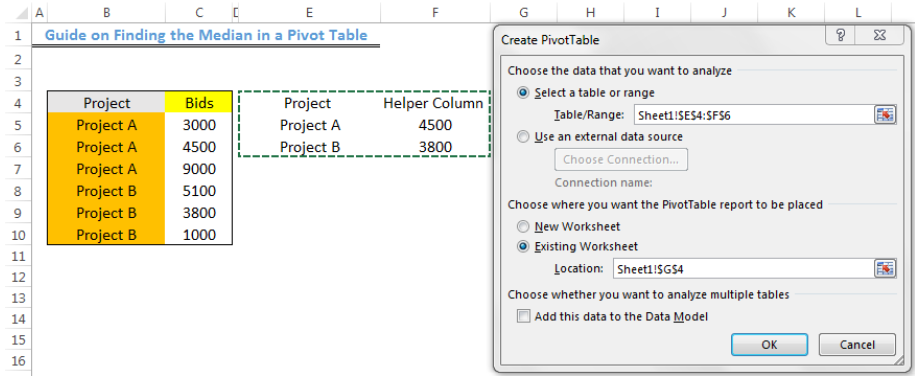 Figure 5- Creating the Pivot Table
- We will press OK
- We will check the PROJECT and HELPER COLUMN boxes
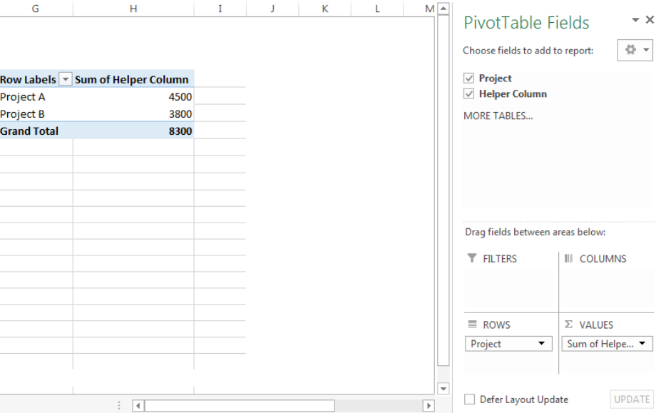 Figure 6- Checking the Project and Helper Column boxes
- We will click on SUM OF HELPER COLUMN and change it to Median Bid
 Figure 7- Median in a Pivot Table
Explanation
=MEDIAN(IF($B$5:$B$10=E5,$C$5:$C$10))
In this formula, the IF function checks the range (B5:B10) for cells that have values equal to E5 (Project A). The identified cells are matched with the corresponding cell in Column C and this is returned to the MEDIAN function.
The MEDIAN function returns the middle number for an odd number of values and averages the two middle numbers for an even number of values as the result.
Instant Connection to an Expert through our Excelchat Service
Most of the time, the problem you will need to solve will be more complex than a simple application of a formula or function. If you want to save hours of research and frustration, try our live Excelchat service! Our Excel Experts are available 24/7 to answer any Excel question you may have. We guarantee a connection within 30 seconds and a customized solution within 20 minutes.


Leave a Comment