How to Apply VLOOKUP with Two Criteria (plus Formula Examples)

While using the VLOOKUP function in Excel, we will often need to lookup a value based on two criteria. This is possible by modifying the lookup value in the standard VLOOKUP function. In this tutorial, we will learn how to apply VLOOKUP with two criteria.

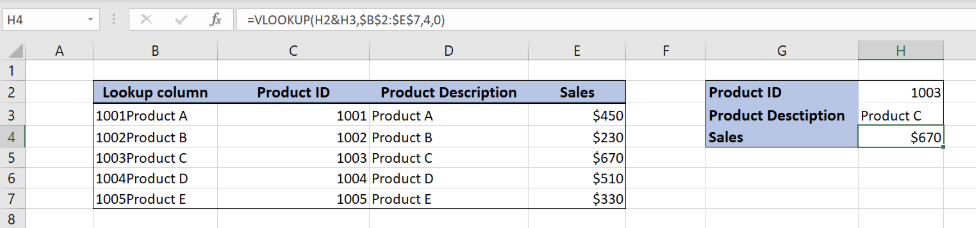
Figure 1. Final result

Syntax of the VLOOKUP formula

The generic formula of VLOOKUP looks like:

=VLOOKUP(lookup_value, table_array, col_index_num, range_lookup)

The parameters of the VLOOKUP function are:

• lookup_value – a value that we want to find in the VLOOKUP table
• table_array – a range in which we want to lookup
• col_index_num – a column number from which we would like to pull a value
• range_lookup – default value 0. This means that we want to find an exact match for a lookup value.

Setting up Your Data

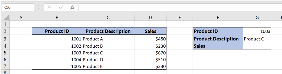Figure 2. Data structure for VLOOKUP with two criteria

In the range B2:D7 we have the table from which we want to pull data. In the cell G4, we want to get Sales value for Product ID 1003 and Product description Product C.

In order to look up into two columns, we have to add one helping columns in the VLOOKUP table. We inserted the column “Lookup column” on the left, where we joined values of columns “Product ID” and “Product Description”.

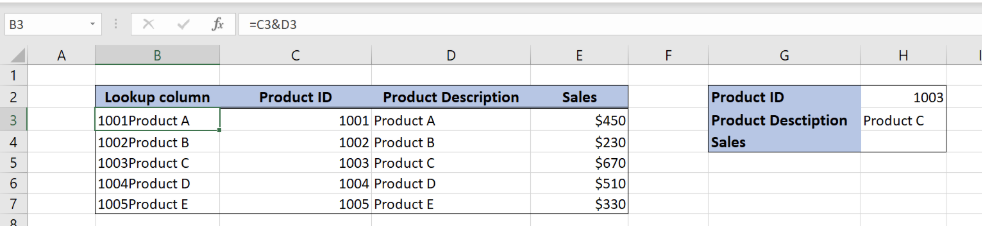Figure 3. Modified data structure for VLOOKUP with two criteria

Modified VLOOKUP formula with two criteria

Now when we have set up our data, our goal is to get the sales value into H4 from the column E, based on values in H2 and H3 cells.

Figure 4. Application of VLOOKUP formula with two criteria

The formula looks like:

=VLOOKUP(H2&H3,$B$2:$E$7,4,0)

In our example, the lookup_value is the combination of cells H2 and H3 (H2&H3). The parameter table_array is $B$2:$E$7 because we want to find value from the range B2:E7. Col_index_num has value 4, as we want to pull value from the 4th column of the range. Finally, range_lookup has value 0, because we want to find an exact match of “Lookup column” values.

To apply VLOOKUP with two criteria, we need to follow these steps:

• Add the helping column at the beginning, joining the first two columns
• Select cell H4 and click on it
• Insert the formula: =VLOOKUP(H2&H3,$B$2:$E$7,4,0)
• Press enter

As a result, we will get $670 in the cell H4. We can see in the VLOOKUP table the sales value for “1003Product C” is $670 in the cell E5.

Most of the time, the problem you will need to solve will be more complex than a simple application of a formula or function. If you want to save hours of research and frustration, try our live Excelchat service! Our Excel Experts are available 24/7 to answer any Excel question you may have. We guarantee a connection within 30 seconds and a customized solution within 20 minutes.