

Excel allows us to lookup two client rates and summarize the sales values based on both rates. This step by step tutorial will assist all levels of Excel users in using double VLOOKUP to get the total sales based on the two client rates.
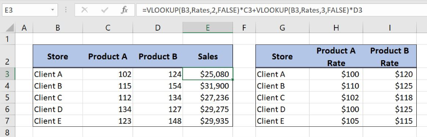 Figure 1. How to Vlookup with two client rates
Syntax of the VLOOKUP formula
The generic formula of VLOOKUP looks like:
=VLOOKUP(lookup_value, table_array, col_index_num, range_lookup)
The parameters of the VLOOKUP function are:
- lookup_value – a value that we want to find in the VLOOKUP table
- table_array – a range in which we want to lookup
- col_index_num – a column number from which we would like to pull a value
- range_lookup – default value 0. This means that we want to find an exact match for a lookup value.
Setting up Our Data to Get Sales Values Based on Two Product Rates per Client
Our first table consists of 4 columns: “Store” (column B), “Product A” (column C), “Product B” (column D) and “Sales” (column E). The second one has three columns: “Store” (Column G), “Product A Rate” (Column H) and “Product B Rate” (Column I). The idea is to get the total sales in Column E based on the sales quantities for products A and B, and respective rates per clients and products.
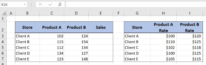 Figure 2. The data structure for VLOOKUP with two client rates
Use VLOOKUP with Two Client Rates
We want to get the sales values per each client based on the different client rates per product. In order to make the formula more clear, we will create a named range Rates for cell range G3:I7.
To create a named range we should follow the steps:
- Select the cell range that should be named
- Click on the name box in Excel
- Write the name for the cell range and press enter
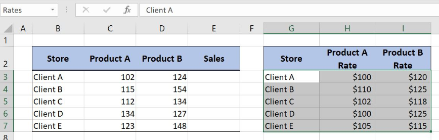 Figure 3. Creating a named range Rates for VLOOKUP table array
The formula looks like:
=VLOOKUP(B3,Rates,2,FALSE)*C3+VLOOKUP(B3,Rates,3,FALSE)*D3
The lookup_value is the cell B3 in both VLOOKUP functions while the parameter table_array is the named range Rates. In the first VLOOKUP function, Col_index_num has value 2, as we want to pull value from the second column of the range, while in the second one this value is 3. Finally, range_lookup has value 0 by default, because we want to find an exact match of “Lookup column” values. VLOOKUP functions are then multiplied with cells C3 and D3 respectively.
To apply the VLOOKUP function we need to follow these steps:
- Select cell E3 and click on it
- Insert the formula:
=VLOOKUP(B3,Rates,2,FALSE)*C3+VLOOKUP(B3,Rates,3,FALSE)*D3 - Press enter
- Drag the formula down to the other cells in the column by clicking and dragging the little “+” icon at the bottom-right of the cell.
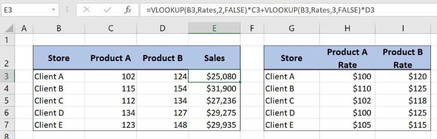 Figure 4. Application of the VLOOKUP formula to get sales values based on two rates
The result of the first VLOOKUP function is the Product A rate per client while the result of the second VLOOKUP is the Product B rate. Rates are then multiplied with sales quantities per each product. The sum of the Product A and Product B sales is the final result placed in column E.
Most of the time, the problem you will need to solve will be more complex than a simple application of a formula or function. If you want to save hours of research and frustration, try our live Excelchat service! Our Excel Experts are available 24/7 to answer any Excel question you may have. We guarantee a connection within 30 seconds and a customized solution within 20 minutes.


Leave a Comment