

VLOOKUP is one of the most used functions for lookup in Excel. One of the shortcomings of this function is it only works for looking up data having a single criterion. Yet, with a simple workaround, we can make VLOOKUP work with multiple criteria. In this tutorial, we will learn to use VLOOKUP with multiple criteria.
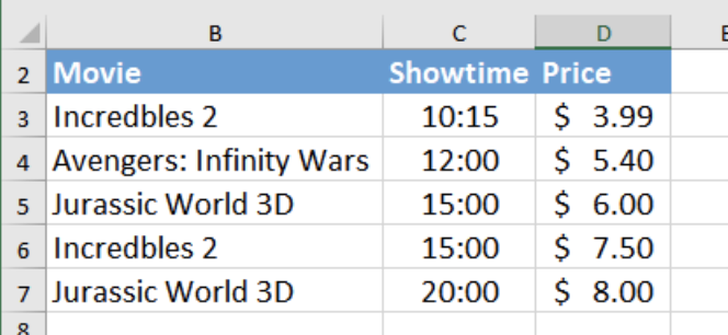 Figure 1. Data set for VLOOKUP with Multiple Criteria
Syntax for Using VLOOKUP with multiple criteria
VLOOKUP formula:
=VLOOKUP(lookup_value, table_array, col_index_num, [rng_lookup])
The VLOOKUP formula fails to look up data having multiple criteria. VLOOKUP with multiple criteria is looking for data including several criteria. We need to make some modifications for it
to work with multiple criteria. The formula will now be,
=VLOOKUP(lookup_val1&lookup_val2, table_array, col_index, [range_lookup])
Setting Up Data
Let’s assume we have a movie theatre data set. It has several unique columns such as the movie names, showtime and ticket prices.
Looking at the data in B2 to C7, we can see that the movie in B11- “Jurassic World 3D” has two records. The price for the first show at 15:00 costs $6.00. The next show at 20:00 costs $8.00.
If we tried to find the price for the premiere at 20:00 with the formula “=VLOOKUP(B11, $B$3:$D$7, 3, FALSE)”, it will show the wrong result. To find the results for multiple criteria using VLOOKUP, we need to make some changes to the formula.
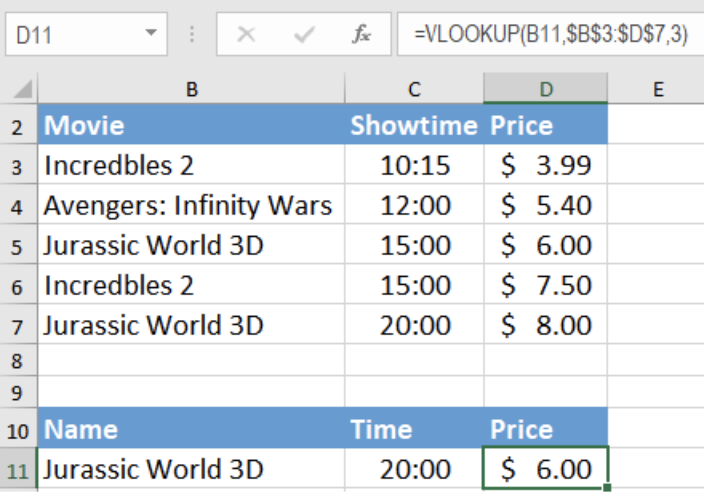 Figure 2. Incorrect Result with VLOOKUP with Single Criterion
The Concatenate Operator(“&”) offers great help to use VLOOKUP with multiple criteria. Before using the concatenate operator, VLOOKUP could not return the correct price for the second show. It did not meet the two criteria( i.e. the Movie name and Showtime).
With help of the concatenate operator, we have specified the two criteria inside the formula. Now, it extracts the correct price for the second show. However, we still have to make sure the range_lookup for VLOOKUP is set to the default value which is TRUE.
To find the correct price for “Jurassic World 3D” at 20:00, we have to :
- Select cell D11 by clicking on it.
- Insert the formula “
=VLOOKUP(B11&C11,$B$3:$D$7,3)”.
- Press Enter.
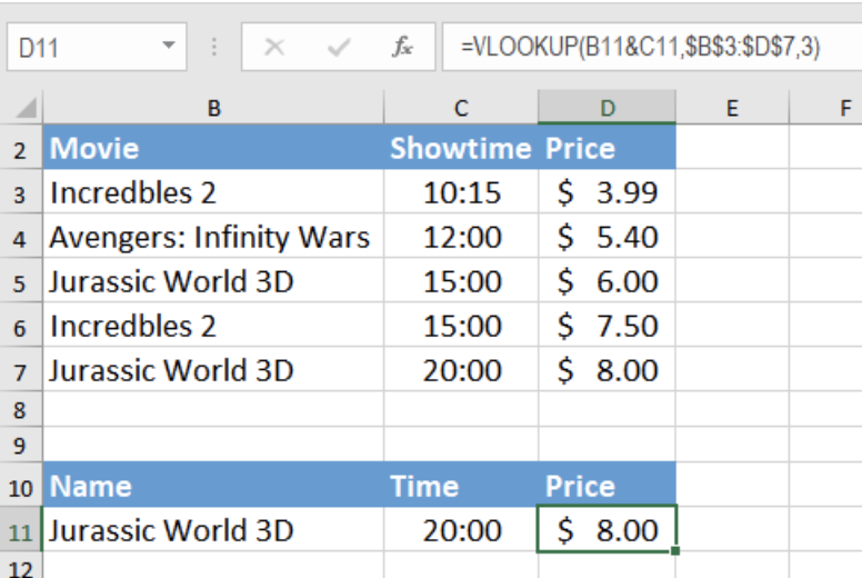 Figure 3. Example of How to use VLOOKUP with Multiple Criteria
This will return the result $8.00 this time. We can be certain that this is the accurate price for the movie “Jurassic World 3D” at “20:00” by matching it with cell D7.
This formula allows us to combine several criteria and use them as one in the VLOOKUP function. It is an easy solution for getting the desired result with several criteria.
Instant Connection to an Expert through our Excelchat Service
Most of the time, the problem you will need to solve will be more complex than a simple application of a formula or function. If you want to save hours of research and frustration, try our live Excelchat service! Our Excel Experts are available 24/7 to answer any Excel question you may have. We guarantee a connection within 30 seconds and a customized solution within 20 minutes.
Are you still looking for help with the VLOOKUP function? View our comprehensive round-up of VLOOKUP function tutorials here.


Leave a Comment