VLOOKUP vs. HLOOKUP: When to Use Each Formula

While working in Excel, we often need to get a value from a table based on a specific value. In this tutorial, we will compare the VLOOKUP and HLOOKUP functions and walk through examples of the when to use each

Syntax of the VLOOKUP formula

The generic formula for the VLOOKUP function is:

=VLOOKUP(lookup_value, table_array, col_index_num, range_lookup)

The parameters of the VLOOKUP function are:

• lookup_value – a value that we want to find in a table_array
• table_array – a range in which we want to lookup
• col_index_num – a column number in table_array from which we would like to get a value
• range_lookup – default value 0. This means that we want to find an exact match for a lookup value.

Setting up Our Data for the VLOOKUP Function

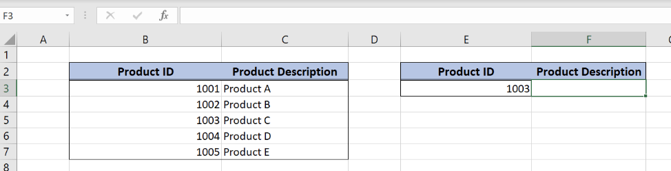Figure 1. Data that we will use in the VLOOKUP example

In this example, our data is organized vertically, so we will use the VLOOKUP function. In the range B2:C7 we have a table from which we want to pull data, while in in the cell F3 we want to get a value. Tables consist of the columns “Product ID” and “Product Description”.

Get the Product description using the VLOOKUP function

Our goal is to obtain data from the “Product Description” column in the second table and populate it into the cell F3.

Figure 2. Using the VLOOKUP function

The formula looks like:

=VLOOKUP(E3, $B$3:$C$7, 2, 0)

In our example, the lookup_value is the E3 cell in “Product ID” column. The parameter table_array is $B$3:$C$7 because we want to find value from the range B3:B7. Col_index_num has value 2, as we want to pull value from the second column of the range. Finally, range_lookup has value 0, because we want to find an exact match of “Product ID” values.

As a result, we will get Product C in the cell F3. As you can see, the value of “Product Description” in C3 in the 1st table is Product C. The function pulls this value and returns it to the cell F3 as a result.

To apply the VLOOKUP function, we need to follow these steps:

• Select cell F3 and click on it
• Insert the formula: =VLOOKUP(E3, $B$3:$C$7, 2, 0)
• Press enter

Syntax of the HLOOKUP formula

The generic formula for the HLOOKUP function is:

=HLOOKUP(lookup_value, table_array, row_index_num, range_lookup)

The parameters of the HLOOKUP function are:

• lookup_value – a value that we want to find in a table_array
• table_array – a range in which we want to lookup
• row_index_num – a row number in table_array from which we would like to get a value
• range_lookup – default value 0. This means that we want to find an exact match for a lookup value.

Setting up Your Data for the HLOOKUP Function

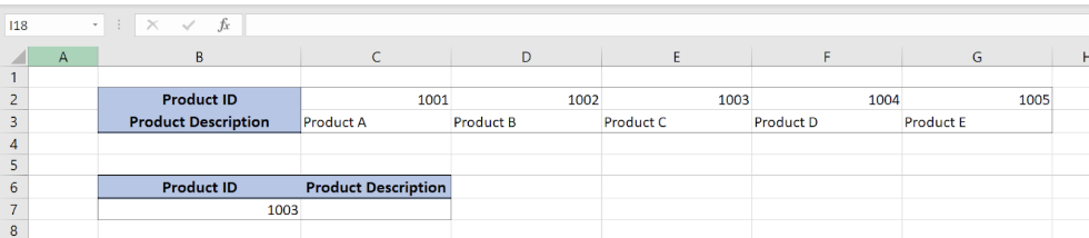Figure 3. Data that wçe will use in the HLOOKUP example

In this example, our data is organized horizontally, so we will use the HLOOKUP function. In the range B2:G3 we have a lookup table, while in in the cell C7 we want to get a value. Tables consist of the rows “Product ID” and “Product Description”.

Get the Product description using the VLOOKUP function

Our goal is to obtain data from the “Product Description” row in the second table and populate it into the cell C7.

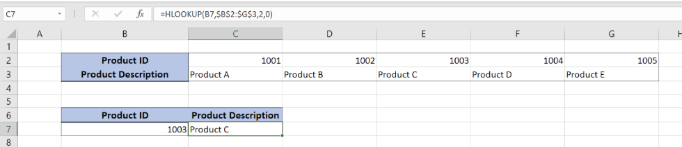Figure 4. Using the HLOçOKUP function

The formula looks like:

=HLOOKUP(B7,$B$2:$G$3,2,0)

In our example, the lookup_value is the B3 cell in “Product ID” column. The parameter table_array is $B$2:$G$3 because we want to find value from the range B2:G3. Row_index_num has value 2, as we want to pull value from the second row of the range. Finally, range_lookup has value 0, because we want to find an exact match of “Product ID” values.

As a result, we will get Product C in the cell C7. As you can see, the value of “Product Description” in E3 in the 1st table is Product C. The function pulls this value and returns it to the cell C7 as a result.

To apply the HLOOKUP function, we need to follow these steps:

• Select cell C7 and click on it
• Insert the formula: =HLOOKUP(B7,$B$2:$G$3,2,0)
• Press enter

Most of the time, the problem you will need to solve will be more complex than a simple application of a formula or function. If you want to save hours of research and frustration, try our live Excelchat service! Our Excel Experts are available 24/7 to answer any Excel question you may have. We guarantee a connection within 30 seconds and a customized solution within 20 minutes.

Are you still looking for help with the VLOOKUP function? View our comprehensive round-up of VLOOKUP function tutorials here.