Using VLOOKUP to Retrieve Information from Different Excel Files

After generating a Pivot Table, you can retrieve specific data from the Pivot Table using the VLOOKUP and GETPIVOTDATA functions. When you use any of these functions, you are basically trying to find your lookup-value on another location in the Pivot Table and retrieve specific information related to that value. The functionality of both features is more or less the same but their syntax is different.

VLOOKUP function on Pivot Table

The Excel VLOOKUP function can be used to retrieve information from a Pivot Table based on cell references. The VLOOKUP function is designed to retrieve data in a table organized into vertical rows, so the lookup value must present in the most left-sided column and the targeted value to be retrieved can be in any column to the right, which is called “ column index”.

Syntax

=VLOOKUP (lookup_value, table, col_index, [range_lookup])

In this article, suppose we have a dataset of sales records of some famous cigarette brands in five different regions, and we have summarized the sales of each brand in each region in a Pivot Table as shown below.

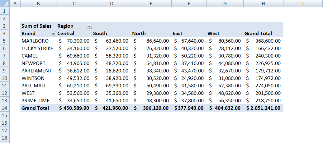
Now, suppose we want to retrieve the summarized sales figure of a specific brand (Lookup value) for a specified region (col_index) from this Pivot Table using the VLOOKUP function.

Here we need to provide the cell references of the lookup-value, pivot table, col_index, and range_lookup to get the resulting information.

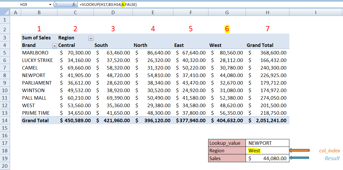
=VLOOKUP (H17, B3:H14, 6, FALSE)

As you can see, we have used following cell reference in this formula

Lookup-value– Cell H17 (NEWPORT) value to look for in the first column of the pivot table

Table – Pivot Table cells range reference B3:H14 as a table from which to retrieve a value.

col_index – WEST region is 6th column in the table from which to retrieve a value.

range_lookup – [optional]

TRUE = approximate match (default).
FALSE = exact match.

If you are using the VLOOKUP function in another worksheet to retrieve the data from the Pivot Table sheet, then this formula will incorporate the Pivot Table sheet name as a reference to the table, like;

=VLOOKUP (H17, Pivot_Table!B3:H14, 6, FALSE)

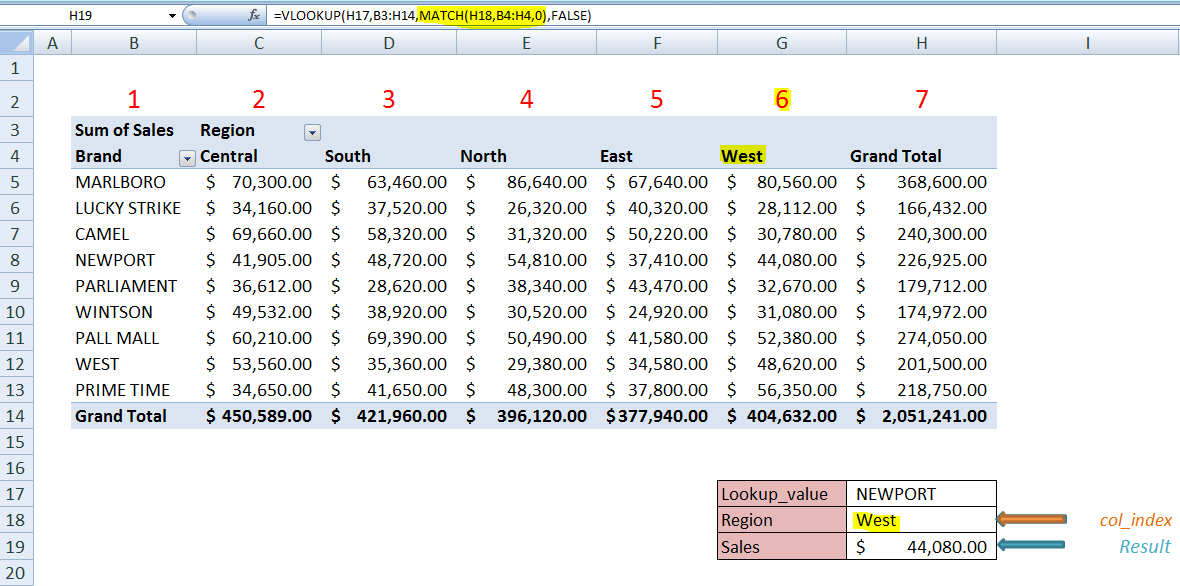
If you want to pick the col_index number automatically with respect to region cell reference, then we can achieve this by introducing MATCH function within VLOOKUP function, like;

=VLOOKUP (H17,B3:H14,MATCH(H18,B4:H4,0),FALSE)

Now the MATCH function will look up for the region cell reference value, as given in cell H18, in column header range of Pivot Table, B8:H4, and will return the column index number where there would be a match. Like, in above example, region “West” is matched in cell G4, so it will return the column index number as 6, because column G is 6th column in Pivot Table range.

The GETPIVOTDATA function on a Pivot Table

The Excel GETPIVOTDATA function retrieves data from a Pivot Table based on Pivot Table structure, instead of cell references. It is a more flexible and dynamic function to get results. You don’t need to remember the syntax and it is generated automatically when you type an equal sign “=”anywhere in worksheet or workbook and click on a value cell as the reference in Pivot Table like you enter this in cell H19

= click on cell F8 in Pivot Table and press ENTER

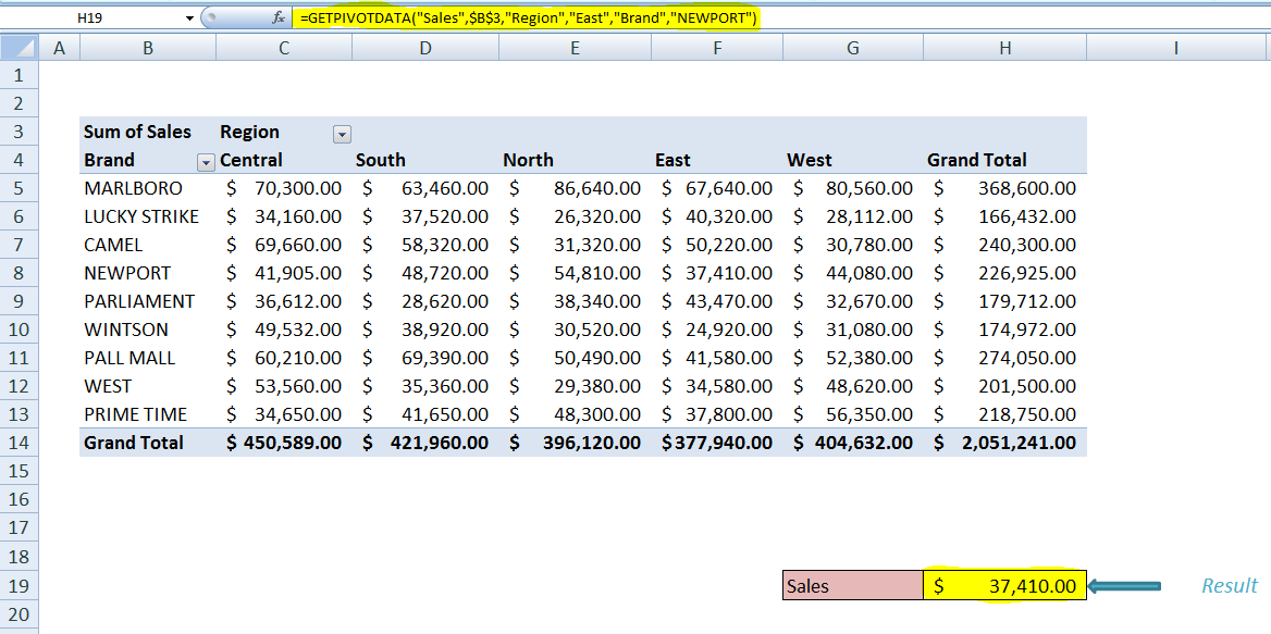
It will automatically generate GETPIVOTDATA function with respect to value cell F8, like this:

=GETPIVOTDATA("Sales",$B$3,"Region","East","Brand","NEWPORT")

However, you can turn off the Generate GetPivotData in the menu at Pivot Table Tools > Options and can create GETPIVOTDATA formula by following its syntax as per your own requirement.

Syntax

=GETPIVOTDATA (data_field, pivot_table, [field1, item1], [field2, item2], ..... )

Where,

data_field – The name of the value field to query.

pivot_table – A reference to the cell where pivot table starts in.

field1, item1 – [optional] – A field/item pair.

These optional field/item pairs are used to limit data retrieval such as applying filters based on pivot table structure. You can limit your results by introducing multiple field/item pairs as per pivot table structure.

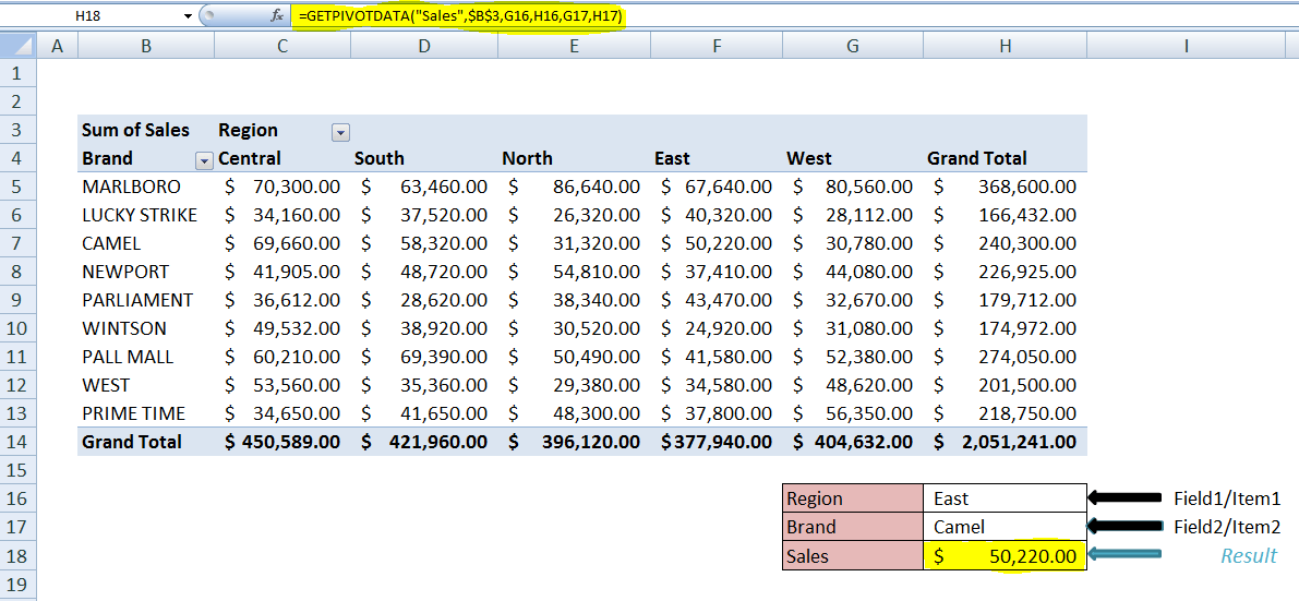
In short, in a GetPivotData formula you refer to the pivot table, and the field(s) and item(s) that you want the data for. In this example, you refer to the pivot table cell $B$3, and want sales data ( data_field) from two field/item pairs, like Region/West and Brand/Camel.

In the formula, data_field must be provided in double quotes, and names of field/item pairs can be in double quotes or you can provide cell references, like the following;

=GETPIVOTDATA("Sales",$B$3,”Region”,”East”,”Brand”,”Camel”) OR =GETPIVOTDATA("Sales",$B$3,G16,H16,G17,H17)

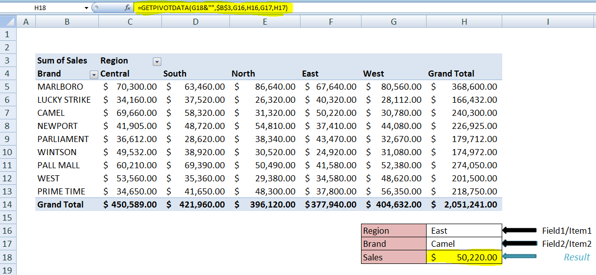
You can also provide data_field as a cell reference, but you need to concatenate it with double quotes in start or end of the cell reference, otherwise, you will get an error in the formula, like this;

=GETPIVOTDATA(G18&"",$B$3,G16,H16,G17,H17)

VLOOKUP vs. GETPIVOTDATA functions

Here are some points which differentiate both functions from each other.

VLOOKUP function is not as flexible as GETPIVOTDATA function.
VLOOKUP function is dependent on the table range reference provided in the formula. It is not effective if the Pivot table range expands. While GETPIVOTDATA is based on the pivot table structure, so it remains effective even if the pivot table expands or collapses.
GETPIVOTDATA function is dynamic and you can extract data from multiple pivot tables which follow same pivot table structure using a single formula. While VLOOKUP function is not dynamic.
In GETPIVOTDATA function you can filter your results by introducing multiple field/item pairs, but it is not possible with VLOOKUP function.

If you haven’t found your answer in this article, our Excel experts are available to help you save hours of researching information. Use this link to type your question and connect to a qualified Excel expert in a few seconds and they will solve your problem on the spot in a live, 1:1 chat session.

Are you still looking for help with the VLOOKUP function? View our comprehensive round-up of VLOOKUP function tutorials here.