

VLOOKUP function is one of the most popular functions in Microsoft Excel. It provides a quick way of looking up a value and retrieving specific data from a table or range. This step by step tutorial will assist all levels of Excel users in the usage and syntax of VLOOKUP function, as well as several applications to everyday work or tasks.
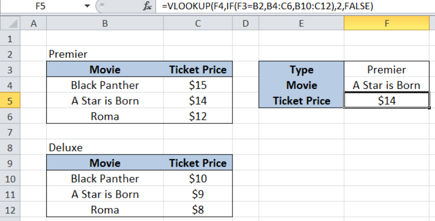 Figure 1. VLOOKUP formula example: VLOOKUP with 2 lookup tables
Syntax of VLOOKUP function
=VLOOKUP(lookup_value, table_array, col_index_num, [range_lookup])
The parameters of the VLOOKUP function are:
- lookup_value – the value that we want to search and find in the table_array
- table_array – the range of cells in the source table containing the data we want to retrieve
- col_index_num – the column number in the table_array corresponding to the information we want to retrieve, relative to the lookup_value
- [range_lookup] – optional; value is either TRUE or FALSE
- if TRUE or omitted, VLOOKUP returns either an exact or approximate match
- if FALSE, VLOOKUP will only find an exact match
In using VLOOKUP, we only need to remember the four needed parameters :
WHAT, WHERE, Column Number, Closest Match
- lookup_value – the WHAT parameter, this is what we want to look for
- table_array – the WHERE parameter, this is where we want to look, where lookup_value can be found in the leftmost column
- col_index_num – the COLUMN NUMBER, this is the column number of the data we want to extract, starting the count from the leftmost column of table_array
- [range_lookup] – the CLOSEST MATCH; if TRUE, we want to find the closest or exact match, if FALSE, we only want to find the exact match
Applications of VLOOKUP
In this article we will learn some useful applications of the VLOOKUP function such as:
- Quickly looking up birthdays of employees
- Calculating grades
- Merging two tables into one
- VLOOKUP with two tables
Quickly look up employee birthday
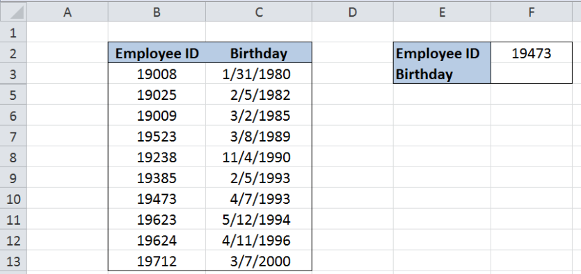 Figure 2. VLOOKUP formula example: Lookup birthdays of employees
Suppose we have a list of employees and their birthdays, the quickest way to lookup the birthday given the employee ID is by using VLOOKUP.
Step 1. Select cell F3
Step 2. Enter the formula: =VLOOKUP(F2,B3:C13,2,FALSE)
Step 3: Press ENTER
As discussed above, VLOOKUP has four parameters. For this example, we want to find F2
(What) in B3:C13 (Where) and obtain 2 (Column Number) using FALSE (Exact Match). The column number is 2 because birthday is in the second column of our table array B3:C13.
As a result, we have found an exact match for Employee ID 19473 along column B, and moving to the second column to the right, obtains the birthday “4/7/1993”.
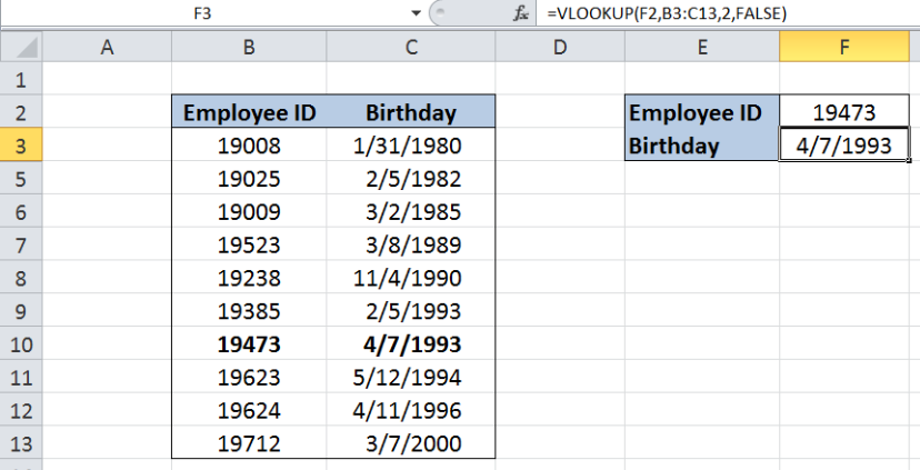 Figure 3. Using VLOOKUP to obtain employee birthday
In just a few seconds, we are able to obtain the birthday of an employee given the employee ID with VLOOKUP. Alternative methods would have been to go through the list one by one, or to filter the list to show employee ID 19473, both of which consumes precious time and are prone to errors.
Calculate grades with VLOOKUP
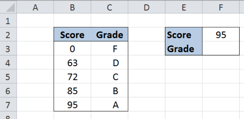 Figure 4. VLOOKUP formula example: Calculate grades with VLOOKUP
Suppose we are given a table with two columns: Cut-off Score (column B) and Grade (column C). We want to be able to quickly determine the equivalent grade for a given score. We can do this with VLOOKUP and using an approximate match.
Step 1. Select cell F3
Step 2. Enter the formula: =VLOOKUP(F2,B3:C7,2,TRUE)
Step 3: Press ENTER
 Figure 5. Using VLOOKUP with exact match to calculate grades
Our VLOOKUP formula searches for the score 95 along column B. Upon finding the score, it then moves to the second column to the right and obtains the grade “A”. Finally, we are able to determine the equivalent grade for 95 using VLOOKUP.
Using an approximate or closest match will allow us to obtain the grade for scores that are not listed in the table B3C8. Let us try and enter 93 into cell F2.
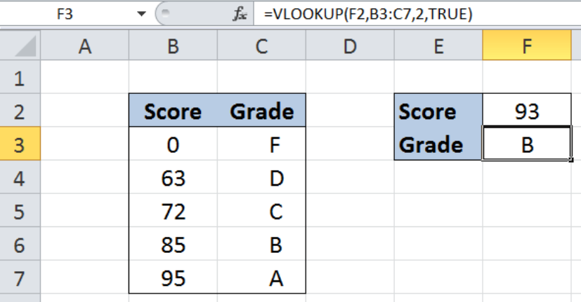 Figure 6. Using VLOOKUP with approximate match to calculate grades
When the formula doesn’t find the lookup_value in the table, it will look for the value closest to but less than the look-up value. In this case, our formula considered score 85 and returned the equivalent grade of B.
If we have used an exact match instead, our formula would have returned an error. See below example:
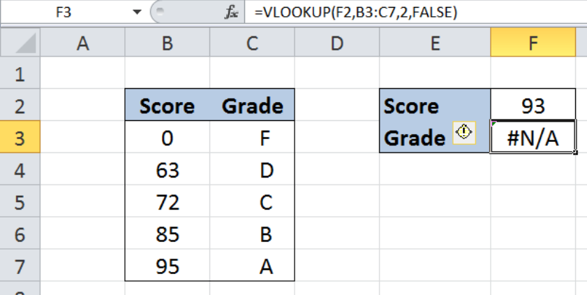 Figure 7. VLOOKUP with exact match returns an error when no match is found
Merging two tables into one
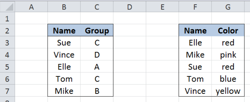 Figure 8. VLOOKUP formula example: Merging two tables into one
Here we have two tables with two columns each. Table 1 contains “Name” and “Group” while Table 2 contains “Name” and “Color”. We want to merge the two tables and come up with a table with three columns: Name, Group and Color.
We can easily merge the two columns by using VLOOKUP with exact match.
Step 1. Add a third column in Table 1 entitled “Color”
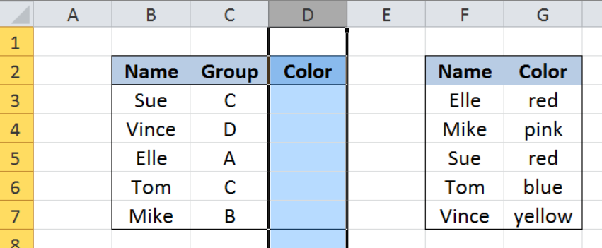 Figure 9. Adding a column to merge two tables
Step 2. Enter this formula in D3: =VLOOKUP(B3,$F$3:$G$7,2,FALSE)
Step 3: Press ENTER
Step 4: Copy the formula in cell D3 to cells D4:D7 by clicking the “+” icon at the bottom-right corner of cell D3 and dragging it down
The dollar signs “$” in the formula fix the cells so that we can easily copy and paste the formula to other cells.
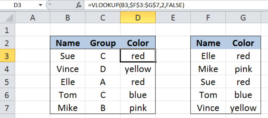 Figure 10. Using VLOOKUP to merge two tables
We have now successfully merged the two tables into one, as shown above in B2:D7.
VLOOKUP with two lookup tables
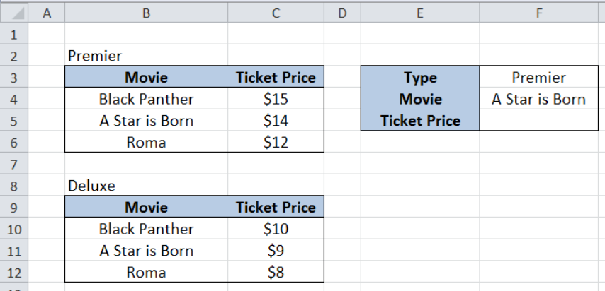 Figure 11. VLOOKUP formula example: VLOOKUP with 2 lookup tables
Suppose we have two tables with two columns each, Movie (column B) and Ticket Price (column C). Table 1 is for “Premier” tickets, while Table 2 is for “Deluxe”. In cells F3 and F4 we enter the criteria for Type and Movie. We want to lookup the movie in the appropriate table and obtain the ticket price. The value for Type will determine which table we will be using in the lookup.
We can use a formula using VLOOKUP and the IF function.
Step 1. Select cell F5
Step 2. Enter formula: =VLOOKUP(F4,IF(F3=B2,B4:C6,B10:C12),2,FALSE)
Step 3: Press ENTER
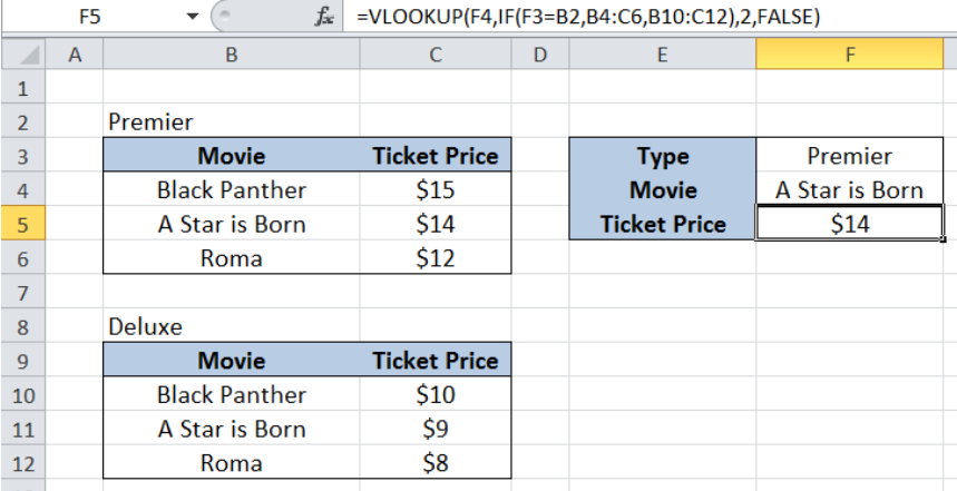 Figure 12. Using VLOOKUP and IF with 2 lookup tables
Our formula searches for “A Star is Born” in the table for “Premier”, B4:B6, and returns the corresponding ticket price of $14. The key here is by combining the VLOOKUP and IF functions. The IF evaluates the type and returns B4:B6 as the table_array if F3 is equal to B2 or “Premier”; otherwise, it returns B10:C12.
The four examples we have learned are just a few of the applications of the VLOOKUP function. VLOOKUP offers a whole lot more, and it has the potential to improve productivity and data handling when mastered and applied everyday.
Most of the time, the problem you will need to solve will be more complex than a simple application of a formula or function. If you want to save hours of research and frustration, try our live Excelchat service! Our Excel Experts are available 24/7 to answer any Excel question you may have. We guarantee a connection within 30 seconds and a customized solution within 20 minutes.


Leave a Comment