How to Use VLOOKUP by Date in Excel

We can find values (numbers or text) that are associated with particular dates in excel by using the VLOOKUP function. We can do this by following the easy steps below.

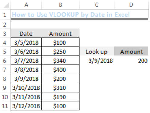Figure 1: The Result of the Lookup Date

Setting up the Data

We need to have a table to make use of the VLOOKUP function. This table will contain the Dates in Column A and the Amounts (this could be text) in Column B.

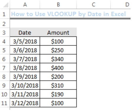Figure 2: Setting up the Data

Syntax

=VLOOKUP(lookup_value,table_array,col_index_number,{range_lookup})

Explanation

• Lookup Value

This is the particular date that we are interested in. For instance, if we are interested in 3/9/2018, our Lookup Value will be A8 because that date is in Cell A8.

• Table Array

This is the range of values from where we will retrieve our value contained in the data. It is noteworthy that we must have at least two columns of data. Our range, in this case, is A4:B11.

• Column Index Number

This is the number of columns from where we will retrieve our data. In this case, we have just two columns, hence, our column index number is 2.

• Range Lookup

This will return values as TRUE or FALSE. TRUE means that we want an approximate match for the selected date and FALSE implies that we want an exact match. We will opt for an exact match.

Look up Value for 3/9/2018

We will name a Cell that will contain the date and have an empty cell where our formula will return our lookup value.

• Cell C5 will be called lookup
• Cell D5 will be called amount
• Cell C6 will contain the lookup date
• Cell D6 is where we will input our formula

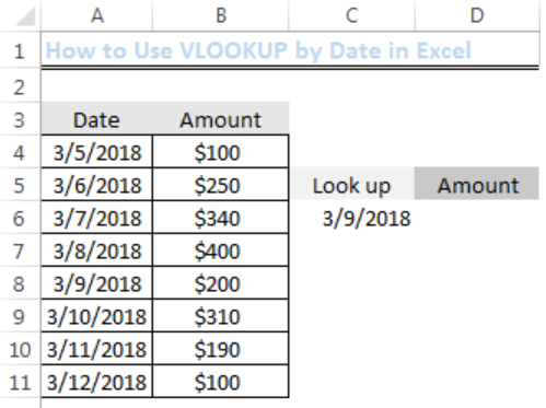Figure 3: Using the VLOOKUP function

Based on the explanation of the syntax above, our formula for 3/9/2018 is:

=VLOOKUP(C6,A4:B11,2,FALSE)

We will input this formula into Cell D6

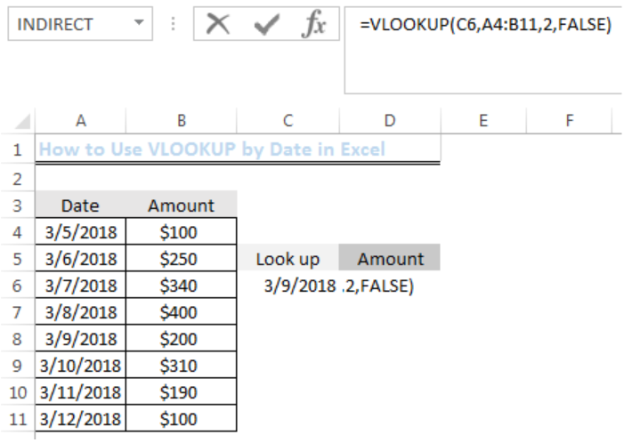Figure 4: Inserting the VLOOKUP function

We will now press ENTER to get the result.

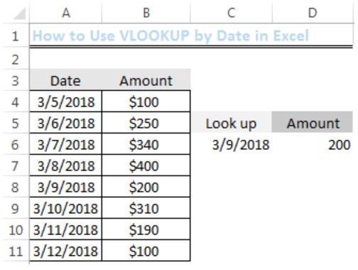Figure 5: Result of the VLOOKUP

The result has provided the amount for the selected lookup date as shown in figure 5.

When using this function, the dates in the table array and the date in the lookup value must be valid.

Instant Connection to an Expert through our Excelchat Service

Most of the time, the problem you will need to solve will be more complex than a simple application of a formula or function. If you want to save hours of research and frustration, try our live Excelchat service! Our Excel Experts are available 24/7 to answer any Excel question you may have. We guarantee a connection within 30 seconds and a customized solution within 20 minutes.

Are you still looking for help with the VLOOKUP function? View our comprehensive round-up of VLOOKUP function tutorials here.