

While working with Excel, we are able to lookup a value and retrieve data from a data set using the VLOOKUP function. VLOOKUP provides a quick way of looking up a value from any list or range. This step by step tutorial will assist all levels of Excel users to lookup the corresponding cost of a specific product using VLOOKUP.
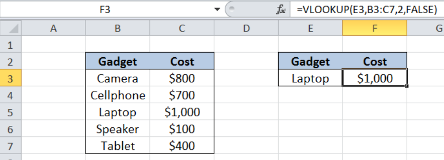 Figure 1. Final result: Lookup cost for product “Laptop”
Final formula: =VLOOKUP(E3,B3:C7,2,FALSE)
Syntax of the VLOOKUP function
=VLOOKUP(lookup_value, table_array, col_index_num, [range_lookup])
The parameters of the VLOOKUP function are:
- lookup_value – the value that we want to search and find in the table_array
- table_array – the range of cells in the source table containing the data we want to retrieve
- col_index_num – the column number in the table_array corresponding to the information we want to retrieve, relative to the lookup_value
- [range_lookup] – optional; value is either TRUE or FALSE
- if TRUE or omitted, VLOOKUP returns either an exact or approximate match
- if FALSE, VLOOKUP will only find an exact match
Setting up Our Data
Here we have a list of Gadgets (column B) and the corresponding Cost (column C). In cell E3, we enter the gadget whose cost we want to look up from our data B2:C7. In this case, let us look up the cost for “Laptop” and record it in cell F3.
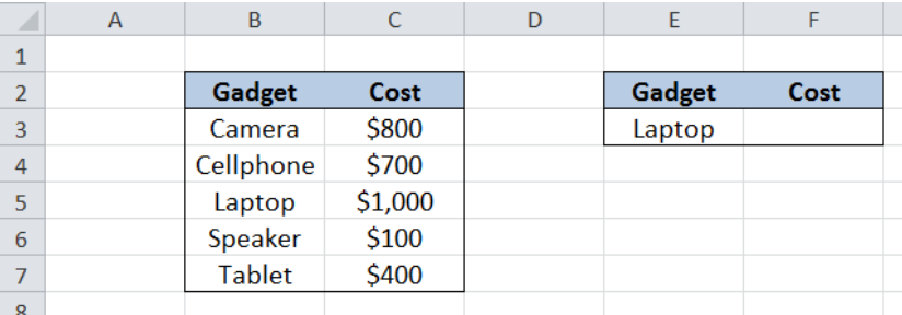 Figure 2. Sample data to lookup cost for product or service
Lookup cost for product “Laptop”
We want to determine the cost for the product “Laptop” without having to search the whole list. In order to lookup a value using VLOOKUP, we follow these steps:
Step 1. Select cell F3
Step 2. Enter the formula: =VLOOKUP(E3,B3:C7,2,FALSE)
Step 3: Press ENTER
Our lookup_value is cell E3, which contains the specific product we want to search: “Laptop”. Our table_array is the range B3:C7. “Cost” is in the second column of the table array so col_index_num is 2. Range_lookup is FALSE because we want to find the exact match.
The final result in cell F3 is $1000, which is the cost of the product we want to search, “Laptop”.
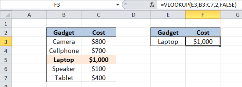 Figure 3. Entering the formula to lookup the cost for “Laptop”
Most of the time, the problem you will need to solve will be more complex than a simple application of a formula or function. If you want to save hours of research and frustration, try our live Excelchat service! Our Excel Experts are available 24/7 to answer any Excel question you may have. We guarantee a connection within 30 seconds and a customized solution within 20 minutes.
Are you still looking for help with the VLOOKUP function? View our comprehensive round-up of VLOOKUP function tutorials here.


Leave a Comment