INDEX MATCH versus VLOOKUP: How and When to Use

VLOOKUP in Excel is a very useful function used for lookup and reference. It looks for the desired values from one row to another to find a match. Using a combination INDEX and MATCH, we can perform the same operations as VLOOKUP. INDEX returns the value of a cell in a table based on the column and row number. MATCH returns the position of a cell in a row or column. Combining these two functions we can look up a value both horizontally and vertically. In this tutorial, we will look the differences between VLOOKUP and INDEX MATCH and when and how to use them.

VLOOKUP uses the syntax :=VLOOKUP(value, table_array, col_index,[range_lookup]).

Why use INDEX MATCH instead of VLOOKUP?

Using INDEX MATCH instead of VLOOKUP is preferred by many Excel professionals. VLOOKUP has many limitations. You can overcome these by using INDEX MATCH. You may use VLOOKUP when the data is relatively small and the columns will not be inserted/deleted. But in other cases, it is best to use a combination of INDEX and MATCH functions. You use the following syntax using INDEX and MATCH together: =INDEX(range, MATCH(lookup_value, lookup_range, match_type)). The main advantages of using INDEX MATCH than VLOOKUP are:

Dynamic Column Reference

The main difference between VLOOKUP and INDEX MATCH is in column reference. VLOOKUP requires a static column reference whereas INDEX MATCH requires a dynamic column reference. With VLOOKUP you need to manually enter a number referencing the column you want to return the value from. As you are using a static reference, adding a new column to the table breaks the VLOOKUP formula. INDEX MATCH allows you to click to choose which column you want to pull the value from. This leads to fewer errors.

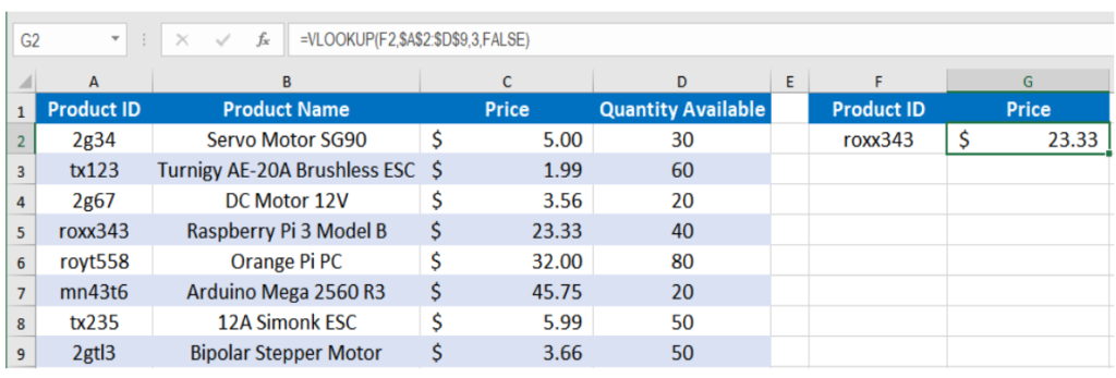
To find the price from the Product ID, select the cell G2 and assign the formula =VLOOKUP(F2,$A$2:$D$9,3,FALSE). Click OK to apply the formula to cell G2 which would show the price for the product in cell F2.

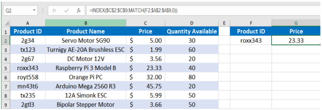
To get the same result using INDEX MATCH, you need to apply the formula =INDEX($C$2:$C$9,MATCH(F2,$A$2:$A$9,0)) to cell G2.

2. Insert/Delete Columns Safely

VLOOKUP uses a static column reference. This breaks the formula each time you add/delete a new column. You can manually set the formula to refer the correct column. But it is a lot of work especially when you have a large data set. INDEX MATCH solves this problem by using a dynamic column reference. You can add/delete columns without distorting the array.

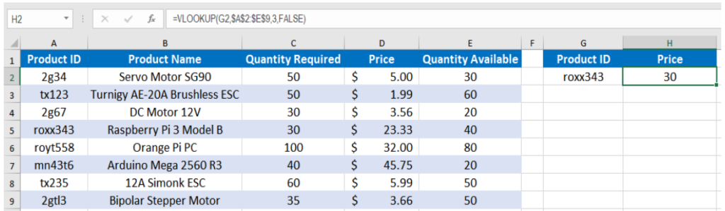
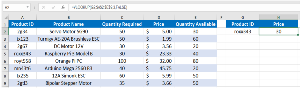
If you add a new column in the previous example named Quantity Required after the Names, the previous formula =VLOOKUP(F2,$A$2:$D$9,3,FALSE) for price would return the value for the Quantity Required which is incorrect.

Using INDEX MATCH will always return the price even after adding/deleting rows as you are using a dynamic reference. To use INDEX MATCH you will assign the formula =INDEX($D$2:$D$9,MATCH(G2,$A$2:$A$9,0)) to cell H2.

3. Lookup Value Size Limit

You need to make sure the total length of your lookup criteria should not exceed 255 characters, otherwise you will end up having the #VALUE! error. But INDEX MATCH can lookup values more than 255 characters in length.

If you had a new column QR Code containing the 320 characters QR Codes for the products from the previous example, the formula =VLOOKUP(F2,$A$2:$D$5,4,FALSE) to find the quantity available would result in a #VALUE error.

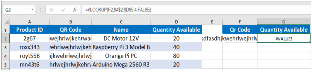
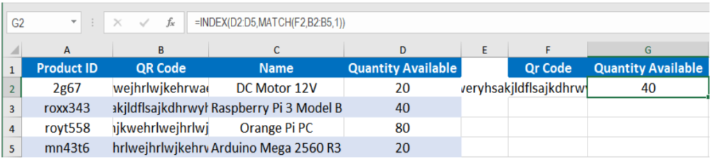
The formula does not work here as the lookup value in cell F2 exceeds 255 symbols. Instead, you need to use the INDEX / MATCH function =INDEX($D$2:$D$5,MATCH(F2,$B$2:$B$5,1)).

4. Higher processing speed

The difference in performances between VLOOKUP and INDEX/MATCH will be negligible if your table_array is small. But if your worksheets contain a lot of rows and formulas, INDEX MATCH will work much faster than VLOOKUP because Excel will have to process only the lookup and return columns rather than the entire table array.

5. Lookup Value Position

VLOOKUP will only work if the lookup value is in the first column. VLOOKUP cannot look to its left. However, INDEX MATCH solves this problem as it performs the lookup both horizontally and vertically. So, it doesn’t require the lookup value to be in the first column, it can be anywhere.

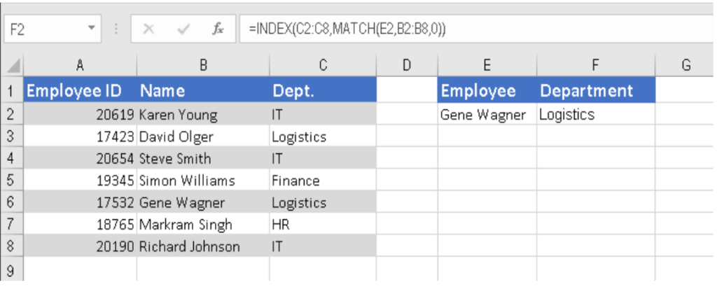
In this example, VLOOKUP fails to return the Dept. looking for name as it is not in the first column. Using INDEX MATCH you can solve this problem. Assign the formula =INDEX(C2:C8,MATCH(E2,B2:B8,0)) in cell F2 and it will return the Dept. Logistics for the employee Gene Wagner.

VLOOKUP assumes by default that the first column in the table array is sorted alphabetically. If your table is not sorted that way, VLOOKUP will return the first closest match which in many cases may not be your desired output. However, INDEX MATCH will return the exact match if it is specified in the formula even if the column for lookup is not sorted.

VLOOKUP is a very effective lookup and reference function. It has some limitations which can be overcome by using INDEX MATCH functions. When you have a small data set and do not have the issues mentioned in this article, you may use VLOOKUP. Otherwise, like most Excel experts, it is best to use INDEX MATCH.

Are you still looking for help with the VLOOKUP function? View our comprehensive round-up of VLOOKUP function tutorials here.