
VLOOKUP function is one of the most popular functions in Microsoft Excel. It is reasonably important to be familiar with the common problems involving VLOOKUP and learning how to solve them. This step by step tutorial will assist all levels of Excel users in solving common VLOOKUP problems.
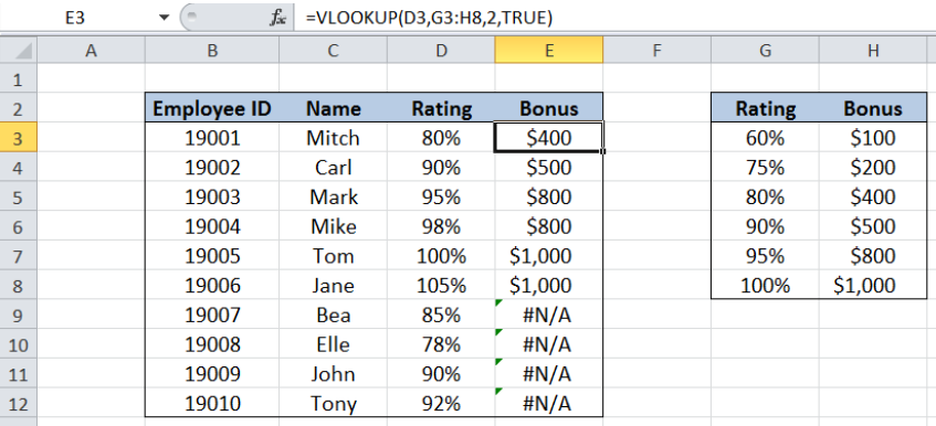 Figure 1. Common VLOOKUP problem: Copying formula without absolute reference
Syntax of VLOOKUP function
=VLOOKUP(lookup_value, table_array, col_index_num, [range_lookup])
The parameters of the VLOOKUP function are:
- lookup_value – the value that we want to search and find in the table_array
- table_array – the range of cells in the source table containing the data we want to retrieve
- col_index_num – the column number in the table_array corresponding to the information we want to retrieve, relative to the lookup_value
- [range_lookup] – optional; value is either TRUE or FALSE
- if TRUE or omitted, VLOOKUP returns either an exact or approximate match
- if FALSE, VLOOKUP will only find an exact match
Common VLOOKUP Problems
In this article we will address some common problems encountered with the VLOOKUP function such as:
- Number entered as text
- Inserting columns
- Wrong use of TRUE or FALSE for range_lookup argument
- Lookup_value not in the first column
- Copying formula without absolute reference
In using VLOOKUP, we only need to remember the four needed parameters :
WHAT, WHERE, Column Number, Closest Match
- lookup_value – the WHAT parameter, this is what we want to look for
- table_array – the WHERE parameter, this is where we want to look, where lookup_value can be found in the leftmost column
- col_index_num – the COLUMN NUMBER, this is the column number of the data we want to extract, starting the count from the leftmost column of table_array
- [range_lookup] – the CLOSEST MATCH; if TRUE, we want to find the closest or exact match, if FALSE, we only want to find the exact match
Setting up our Data
Our table consists of four columns: Employee ID (column B), Name (column C), Rating (column D) and Bonus (column E).
In cells G3:H8, we have a table of ratings with corresponding bonus. We want to lookup the rating and obtain the corresponding bonus per employee by using VLOOKUP. Results will be recorded in column E.
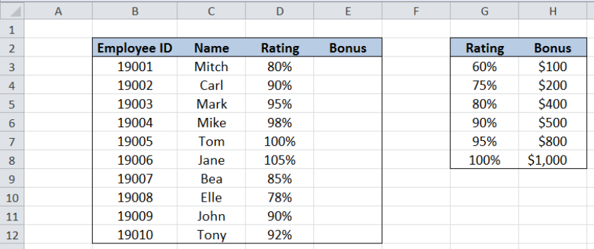 Figure 2. Sample data for common VLOOKUP problems
In order to get the bonus for each employee, we follow these steps:
Step 1. Select cell E3
Step 2. Enter the formula: =VLOOKUP(D3,$G$3:$H$8,2,TRUE)
Step 3: Press ENTER
Step 4: Copy the formula in cell E3 to cells E4:E12 by clicking the “+” icon at the bottom-right corner of cell E3 and dragging it down
The dollar signs “$” in the formula fix the cells so that we can easily copy and paste the formula to other cells.
Our formula looks up the closest match for the rating in column D in the range G3:H8, then moves to the second column to the right and obtains the corresponding grade.
The table below shows the bonus for each employee as supplied by the VLOOKUP function.
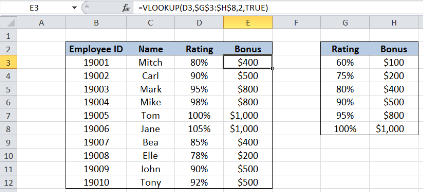 Figure 3. Using VLOOKUP to calculate the bonus per employee
Number entered as text
One common problem with VLOOKUP is when values are mistakenly entered as text. See below example where cell D4 is entered as text, with an apostrophe at the beginning: ‘90%. As a result, the formula cannot find the lookup value in the range G3:H8, and the #N/A error value is returned instead.
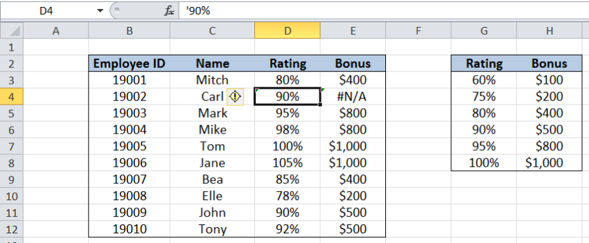 Figure 4. Common VLOOKUP problem: Number entered as text
Work-around:
We can ensure that all values in our table are entered as numbers by following these steps:
Step 1. Select the cells in our table that we want to convert to numbers. In this case, cells D3:D12
Step 2. Click the Data tab, then select Text to Columns
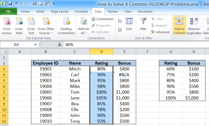 Figure 5. Selecting Text to Columns to convert values to numbers
The Convert Text to Columns Wizard dialog box will pop up.
Step 3: Tick Delimited and click Finish
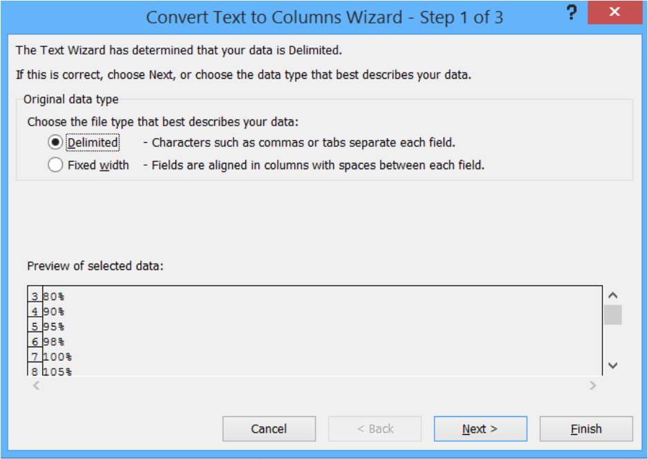 Figure 6. Selecting “Delimited” then “Finish”
We have now converted all the cells in D3:D12 into numbers.
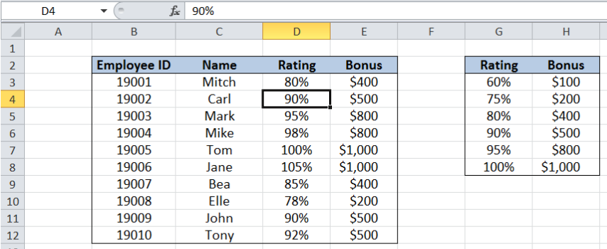 Figure 7. Values converted to numbers using Text to Columns
Inserting columns
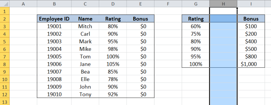 Figure 8. Common VLOOKUP problem: Inserting columns
Another problem encountered with VLOOKUP is when a column or columns are added that affect the cells or range connected with the VLOOKUP formula. See above example where a column is added to the right of column G.
Note that the values for Bonus in column E have all been changed to 0$. Looking closely at the VLOOKUP formula, notice that the value for column index number remains at 2. This means that even if the Bonus column has been moved to column I, which is the third column in the range G3:I8, our formula still refers to the 2nd column.
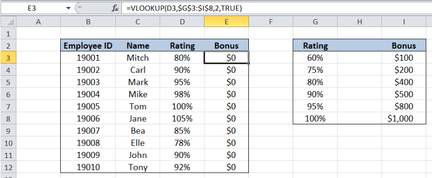 Figure 9. VLOOKUP formula affected with inserted column
Work-around:
We can actually use a the COLUMN function to ensure that the column number will always refer to the appropriate column. Enter the following formula in cell E3:
=VLOOKUP(D3,$G$3:$H$8,COLUMN(H3)-COLUMN(G3)+1,TRUE)
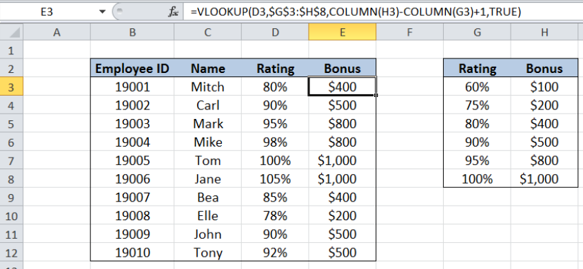 Figure 10. Enhancing VLOOKUP formula as work-around to inserting columns
The COLUMN function subtracts the column numbers of H and G, which is 1, then adds 1, resulting to 2. Now, even if columns are inserted and the column for Bonus is changed, our formula will adapt with the change and still return the correct column number.
Let us copy the formula in cell E3 to cells E4 to E12, then insert a column again to to the right of column G.
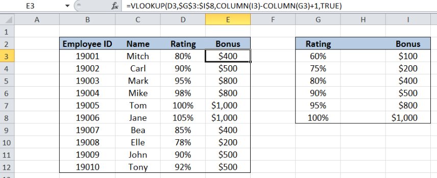 Figure 11. VLOOKUP formula not affected by inserting columns
As shown above, inserting a column didn’t affect the VLOOKUP formula at all. The results in column E remain unchanged.
Wrong use of TRUE or FALSE
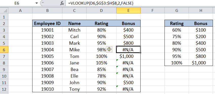 Figure 12. Common VLOOKUP problem: Wrong use of TRUE or FALSE
The table above shows that the range_lookup used in the formula is “FALSE” instead of “TRUE. As a result, the VLOOKUP only searches for a perfect match of the rating. When a rating is not found in G3:H8, the error value #N/A is returned.
Reminder:
The use of TRUE (approximate match) or FALSE (exact match) depends on the requirement of the user.
In this example, we are searching for values in a table with defined ranges or cut-off values. The use of TRUE for an approximate match is necessary. Otherwise, using FALSE for an exact match would return errors for those ratings that fall in between the given cut-off ratings.
Look-up value not in the first column
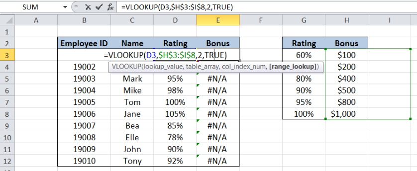 Figure 13. Common VLOOKUP problem: Lookup value not in 1st column
The table above shows that the lookup value in column D containing the rating is not found in the leftmost column of table_array. The range for the table_array has been mistakenly entered as H3:I8 instead of G3:H8.
Reminder :
It is very important to enter the table_array such that the leftmost column is the column where the lookup_value can be found. Otherwise, the VLOOKUP function will return an error value.
Copying formula without absolute reference
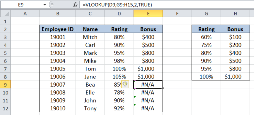 Figure 14. Common VLOOKUP problem: Copying formula without absolute reference
Another common problem encountered with VLOOKUP is dragging cells to copy formulas without fixing the necessary cells for absolute reference. As shown below, cell E9 has the table_array G9:H15, which contains no values. Hence, the formula returns an error because it cannot find the lookup value “85%” in the table_array G9:H15.
In this case, it is absolutely necessary to fix the cells G3:H8 because G3:H8 is the range that contains the data for the ratings and corresponding bonus.
Reminder:
There is a degree of analysis that’s required when creating formulas and copying them to other cells. The cells that serve as references must be fixed with the use of the dollar sign “$” such that copying the formula in any direction would lead to the desired results.
Most of the time, the problem you will need to solve will be more complex than a simple application of a formula or function. If you want to save hours of research and frustration, try our live Excelchat service! Our Excel Experts are available 24/7 to answer any Excel question you may have. We guarantee a connection within 30 seconds and a customized solution within 20 minutes.


Leave a Comment