

While using the standard VLOOKUP function in Excel, a lookup value must be in the leftmost column of a table. In this tutorial, we will learn how to look up for the value even if it is not in the leftmost. In order to do this, we can use the combination of INDEX and MATCH functions or VLOOKUP and CHOOSE function.
Syntax of INDEX and MATCH functions
Firstly, we will explain how to use both of these functions separately. INDEX function returns a value of a particular row in an array. The generic formula looks like:
=INDEX(array, row_num, [col_num])
The parameters of the INDEX function are:
- array – an array in which we want to find a value in a certain position
- row_num – a row number in an array from which we want to take a value
- col_num – a column number in an array from which we want to take a value. This is a non-mandatory parameter.
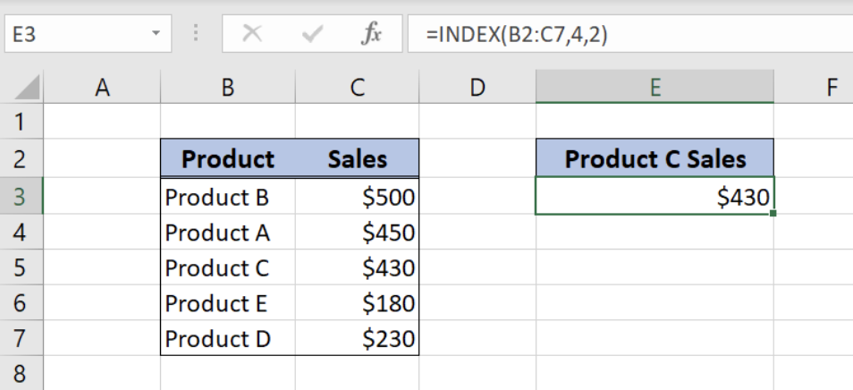 Figure 1. Get the Product C Sales Data from the Table with INDEX function
The MATCH function returns a position of a certain value in an array. The generic formula looks like:
=MATCH(lookup_value, lookup_array, [match_type])
The parameters of the MATCH function are:
- lookup_value – a value which position in an array we want to get
- lookup_array – an array in which we want to find a position of a value
- match_type – a type of match which will be returned. We will use 0 because we want the position of an exact matching value.
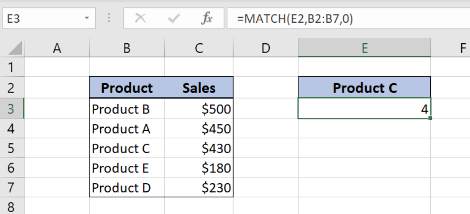 Figure 2. Get the Row Number from the Table Column with MATCH Function
Now, we can look at the generic formula which allows us to look up reference in the left column:
=INDEX(array, MATCH(lookup_value, lookup_array, 0))
The idea is to find a position of a value which we want to find in the lookup array by the MATCH function. Then, we will find a value of that position in the value’s array by INDEX function.
Setting up Your Data
We will now look at the example to explain in details how this formula works. Let’s start with examining the structure of the data that we will use.
The lookup table consists of 3 columns:
- The first column is “Sales” (B),
- The second one is “Product” (C),
- While the third one is “Salesman” (D).
The main table where we want to get data consists of 2 columns:
- The first column is “Product (F),
- The second one is “Sales” (G).
As a result, we want to get Sales value from column B into “Sales” column G, based on “Product” columns match.
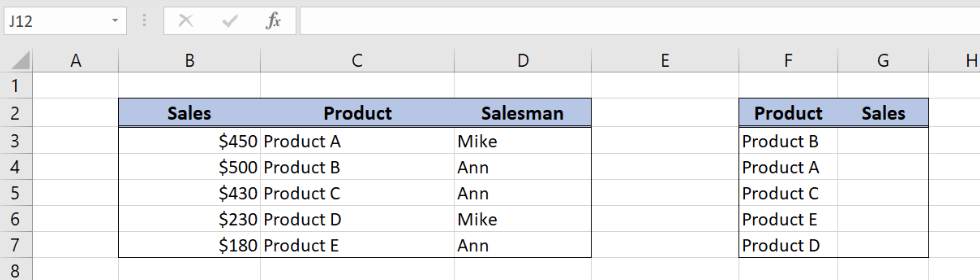 Figure 3. Tables for INDEX and MATCH lookup
Get the Product Sales with INDEX and MATCH
The formula for getting data from the table where lookup array is on the right side looks like:
=INDEX($B$3:$B$7,MATCH(F3,$C$3:$C$7,0))
Let’s look into the MATCH function parameters:
- lookup_value – “Product B” (F3 cell)
- lookup_array – “Product” column in the first table (C3:C7)
- match_type – 0, exact match
As a result of the MATCH function, we will get value 2, as “Product B” is the second in array C3:C7. This value is row_num parameter for the INDEX function.
INDEX function parameters in the example are:
- array – column “Sales” from the first table (B3:B7)
- row_num – result from the match function (value 2)
Column “Sales” from the first table is array in INDEX because we want to get the value of sales from position 2.
To use INDEX and MATCH functions to reference left column, we need to follow these steps:
- Select cell G3 and click on it
- Insert the formula:
=INDEX($B$3:$B$7,MATCH(F3,$C$3:$C$7,0)) - Press enter
- Drag the formula down to the other cells in the column by clicking and dragging the little “+” icon at the bottom-right of the cell.
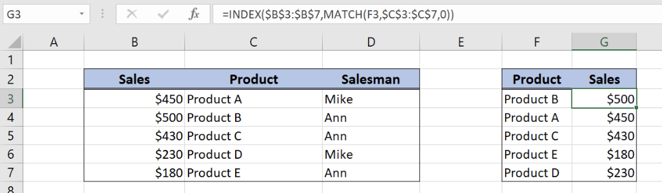 Figure 4. INDEX and MATCH lookup
As a result, we will get $500 in the G3 cell, as “Product B” has position 2 in array C3:C7. Furthermore, position 2 in array B3:B7 has value $500, which is the result of our formula.
An application of VLOOKUP and CHOOSE functions
Firstly, we will explain how to use both of these functions separately. VLOOKUP function looks up for the value and returns the matching value.
The generic formula for VLOOKUP looks like:
=VLOOKUP(lookup_value, table_array, col_index_num, range_lookup)
The parameters of the VLOOKUP function are:
- lookup_value – a value which we want to find in a lookup table
- table_array: – a table in which we want to look up.
- col_index_num – a column number in a lookup table which value we want to pull
- range_lookup – default value 0. This means that we want to find an exact match for a lookup value.
The CHOOSE function can form a table based on given values and positions. First we will explain how the single CHOOSE function works, and how can we use it to change column places in the table.
The generic formula for CHOOSE looks like:
=CHOOSE(index_num, value1, value2, ..., valueN)
The parameters of the CHOOSE function are:
- index_num – position of the value that we want to get
- value1, value2, … – The first, second etc. value from which to choose.
Excel CHOOSE function returns the value from the list, we just have to define a position of that value in the value list.
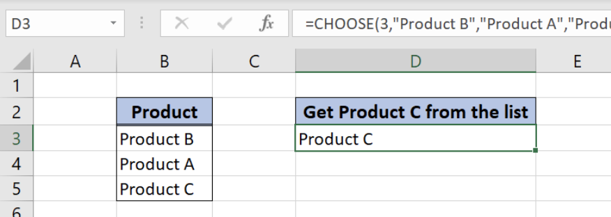 Figure 5. Get the Product C from the table with CHOOSE
For our problem, single CHOOSE function is not very usable. We can use CHOOSE function in combination with VLOOKUP to get the value from the table where lookup array column is on the right side.
Get the value from the table with VLOOKUP and CHOOSE
The idea is to create a table by switching columns position, using CHOOSE function. As a result, the new table (with swapped columns) will be the table_array parameter for VLOOKUP function).
The generic formula which allows us to lookup reference in left column is:
=VLOOKUP(lookup_value, CHOOSE({1,2}, value1, value2), col_index_num, 0)
We will now look at the example to explain in details how this function works. The data structure is the same as in Example 1.
As a result, we want to get Sales value from column B into “Sales” column G, based on “Product” columns match. The idea is to swap positions of columns “Product” and “Sales” in the first table by CHOOSE function. After that, we can use VLOOKUP function in a standard way.
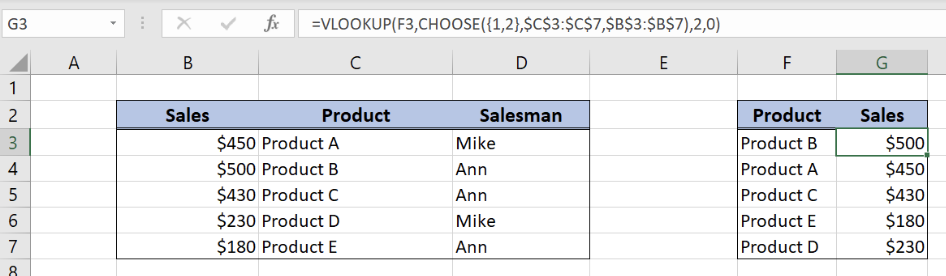 Figure 6. VLOOKUP and CHOOSE lookup
The formula looks like:
=VLOOKUP(F3, CHOOSE({1,2}, $C$3:$C$7, $B$3:$B$7), 2, 0)
- In order to use columns B and C in VLOOKUP, we will swap their positions by CHOOSE function
- The parameter index_num of CHOOSE function has value {1,2}, while the C3:C7 range is value1 and B3:B7 is value2.
- Don’t forget to put index_num values in brackets {} because we are dealing with arrays
This means that the column “Product” will become the first column in the table and the column “Sales” will become the second. A table like this will be the table_array parameter of the VLOOKUP function.
- In VLOOKUP formula, lookup_value is “Product B” (F3 cell).
- Lookup_array is the table from CHOOSE function
- Col_index_num has value 2, as we want to pull value from the second column of the range.
- Finally, range_lookup has value 0, because we want to find an exact match of “Product” values.
To use VLOOKUP and CHOOSE functions to reference left column, we need to follow these steps:
- Select cell G3 and click on it
- Insert the formula:
=VLOOKUP(F3, CHOOSE({1,2}, $C$3:$C$7, $B$3:$B$7), 2, 0) - Press enter
- Drag the formula down to the other cells in the column by clicking and dragging the little “+” icon at the bottom-right of the cell.
As a result, we will get $500 in the G3 cell, as “Product B” has position 2 in array C3:C7. Furthermore, position 2 in array B3:B7 has value $500, which is the result of our formula.
Most of the time, the problem you will need to solve will be more complex than a simple application of a formula or function. If you want to save hours of research and frustration, try our live Excelchat service! Our Excel Experts are available 24/7 to answer any Excel question you may have. We guarantee a connection within 30 seconds and a customized solution within 20 minutes.
Are you still looking for help with the VLOOKUP function? View our comprehensive round-up of VLOOKUP function tutorials here.


Leave a Comment