Excel Fuzzy Lookup Add-In is used to match similar, but not exactly matching data. This function is often used instead of VLOOKUP, when we want to compare two columns which have very similar data, but not exactly the same. As an output, Fuzzy Lookup returns a table of matched similar data in the chosen column. In daily data manipulation, there is a common need to compare two same data sets where one of them comes from some external source and can be misspelled or typed incorrectly. In this tutorial, you will see how to install Fuzzy Lookup Add-In, prepare data and create a Fuzzy Lookup, which can be very useful in data consolidation and save a lot of time.

1.    Installation of Fuzzy Lookup in Excel
2.    Explanation of the function
3.    Preparation of data for Fuzzy Lookup
4.    Create Fuzzy Lookup

1.     Installation of Fuzzy Lookup in Excel

Fuzzy Lookup is not a standard Excel function, therefore you can’t find it in your standard tabs and buttons. In order to enable this function, Microsoft created an Add-In which can be downloaded from the following link:

Download Fuzzy Lookup Add In

After you have downloaded the installation file, you need to open it and install following instructions. Once you have installed the Add-In, next time when you open an Excel it will automatically import Add-In. As a result, you will get a new tab at the end of a Ribbon called “Fuzzy Lookup” and a button with the same name:

2.     Explanation of the function

As mentioned in the intro of the article, Fuzzy Lookup is used when we want to match two sets of data (two tables), but we don’t have exactly the same values in matching fields. For example, we want to match two tables based on values in column “Name” and in a first table we have value “Michael Jackson”, while in a second table we have similar, but misspelled name “Michal Jackson”. In this case, if we use standard VLOOKUP function, it will not match this two values because it’s looking for the exact match. Using of Fuzzy Lookup solves this problem, by matching columns based on their similarity.

This is very often used when we get a table in Excel imported from some other source, or just manually copied and want to match it with another table with the same data sorted out. In most cases, a first table will have many typing mistakes and misspelled words and would first need to be cleaned manually to be able to Lookup it with our prepared table. This can be very time consuming and that’s the point where Fuzzy Lookup saves precious time. Please note that the matching columns must be formatted as text.

3.      Preparation of data for Fuzzy Lookup

Before being able to do a Fuzzy Lookup, we need to format our data into tables. To do this select cells range, click on Insert tab and choose Table. After we have created two tables, they need to be named in order to be used in Fuzzy Lookup function. This is done by selecting the whole table and entering a name into a Name Box:

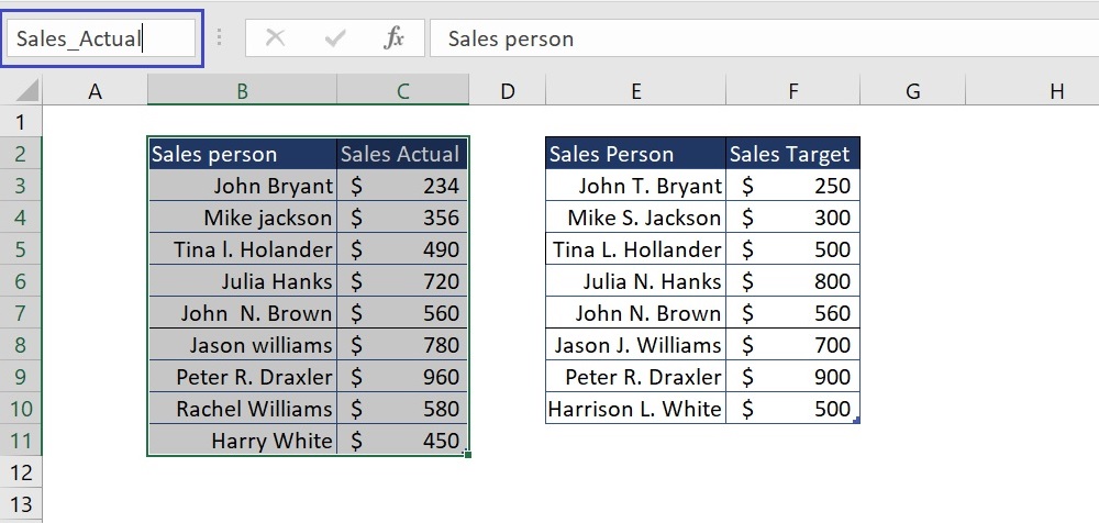
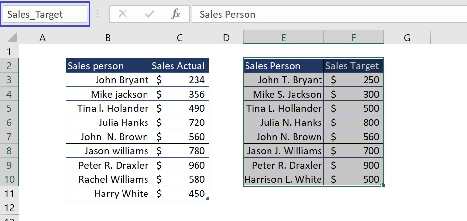
Now we have data ready for Fuzzy Lookup: As you can see on previous pictures, we have two tables: the first one (named Sales_Actual) contains data on actual sales per salesperson (Columns “Sales Person” and “Sales Actual”) and the second one contains data of target sales per salesperson (Columns “Sales person” and “Sales Target”).

4.      Create Fuzzy Lookup

Once we have formatted our data in Spreadsheet, we can start creating Fuzzy Lookup with two tables created. We can imagine that the first table is imported from some other data source and presents a report of sales per sales person, while the second table contains arranged table created in our Excel file which contains targeted sales for every person. In our example, we want to match these two tables based on column “Sales Person” and create a new table which will have all data aggregated (“Sales Person”, “Sales Actual”, “Sales Target”). We can see that the first table has some misspelled names and we want to match them with correct names in the second table based on their similarity.

Let’s now create an example of Fuzzy Lookup and explain how it works. First, we need to select a cell, which will be the first cell of a newly created table, then go to Fuzzy Lookup tab and click on Fuzzy Lookup button. We will get the following window opened on the right side:

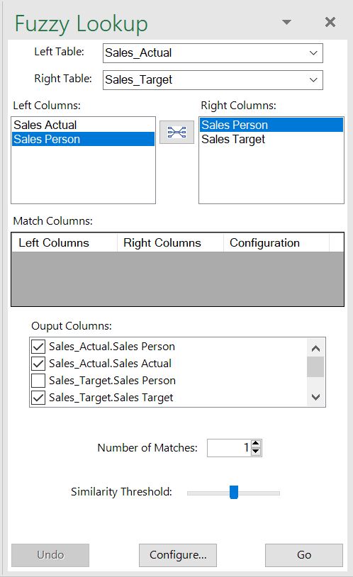
To create our table, we have several steps to do:

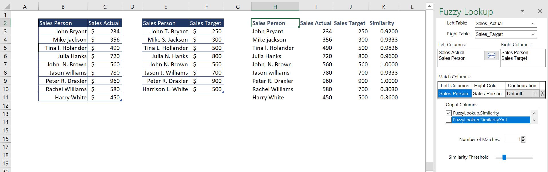
In the first part of Fuzzy Lookup window, we need to choose two tables which will be matched. In our case left table will be “Sales_Actual” and the right table will be “Sales_Target”. After that, we need to choose the columns which we want to match and click on the button between them. In our example, we want to match tables based on similarity of columns “Sales Person”, so we will choose this column both in Left Columns and Right Columns. Once we do that, the table below will have one new row with these matching columns. In Output columns, we need to check columns that we want to be in a newly generated table: “Sales_Person”, “Sales_Actual” and “Sales_Target”.

There is also an option to choose field “FuzzyLookup.Similarity” which gives the percentage of similarity between two columns. In the end, we can choose Similarity Threshold (0-100%) which tells the function what level of similarity we want to match. After everything is set up, we can click go and get a table based on entered parameters:

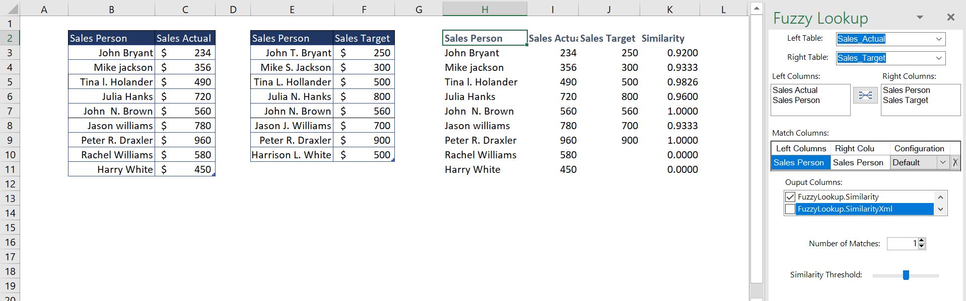
As you can see in the picture, the new table is created from the first two chosen. It consists of 3 columns that we choose and column similarity which calculates the similarity of “Sales_Person” columns in the two tables in percentage. For example, “John Bryant” from the first table is matched with “John T. Bryant” from the second table as their similarity is equal to 92%. Also, names “Rachel Williams” and “Harry White” do not have similar values in the second table (based on similarity percentage – 50%), so no value is filled in “Sales Target” column for these two entries.

If we wanted to get these two values also in the matched table, we would have put smaller Similarity Threshold in Fuzzy Lookup window. In the following example, we put it at 0.2 (20%) which means that we want to match all names that have the similarity of 20% or greater. Here is the result:

The output now is the same table, but with included names “Rachel Williams” and “Harry White” because their similarity to “Jason J. Williams” and “Harrison L. White” is greater than 20%.

Are you still looking for help with the VLOOKUP function? View our comprehensive round-up of VLOOKUP function tutorials here.