

Excel provides us with different methods to compare two columns and find unique or duplicate values with the use of the VLOOKUP, MATCH, INDEX, IF, COUNTIF or Conditional Formatting functions. This step by step tutorial will assist all levels of Excel users in comparing two columns in Excel or Google sheets.
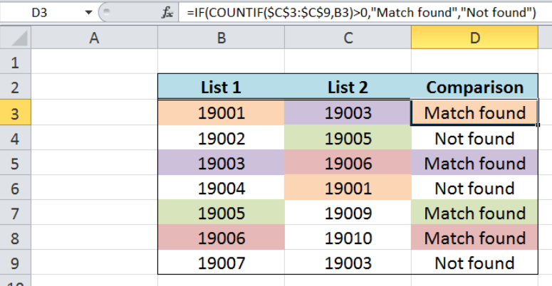 Figure 1. Final result: Compare two columns in Excel
Data to compare two columns in Excel
Our data consists of three columns: List 1 (column B), List 2 (column C) and Comparison (column D). We want to compare the product codes in the two columns B and C. The results of comparison will be recorded in column D.
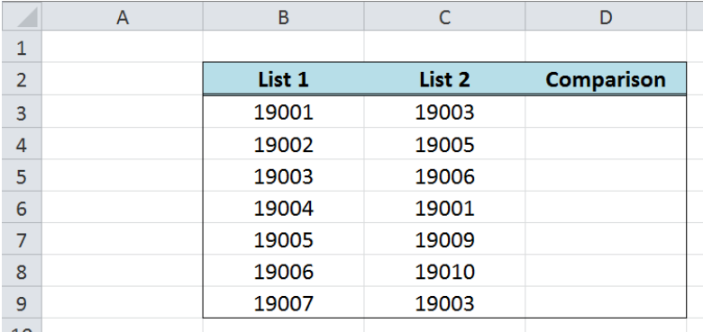 Figure 2. Sample data to compare two columns in Excel
Compare two columns in Excel using VLOOKUP
VLOOKUP is used when we want to look up a value in one column and determine if it exists in another column. There are two match types: approximate match or exact match. When comparing lists, the exact match is most commonly used.
Syntax of the VLOOKUP function
=VLOOKUP(lookup_value, table_array, col_index_num, [range_lookup])
- lookup_value – the value that we want to find in the table_array
- table_array – the range of cells containing the data we want to find or retrieve
- col_index_num – the column number in the table_array corresponding to the information we want to retrieve, relative to the lookup_value
- [range_lookup] – optional; value can either be TRUE or FALSE
- if TRUE or omitted, VLOOKUP returns either an exact or approximate match
- if FALSE, VLOOKUP will only find an exact match
In order to determine if a value in the first column (List 1) exists in another column (List 2) and return the value itself, we follow these steps:
Step 1. Enter the formula in cell D3: =VLOOKUP(B3,$C$3:$C$9,1,FALSE)
Step 2. Press ENTER
Step 3: Copy the formula in cell D3 to cells D4:D9 by clicking the “+” icon at the bottom-right corner of cell D3 and dragging it down
Our lookup_value is the value in column B (B3), while our table_array is the set of values in column C, $C$3:$C$9. The col_index_num is 1, which returns the value in the first column relative to the table_array if the value in column B is found in column C. Otherwise, the function will return the value “#N/A”. The range_lookup is FALSE, which means that the function will look for an exact match.
As a result, the value in cell D3 is “19001”, because the value in column B “19001” is found in column C.
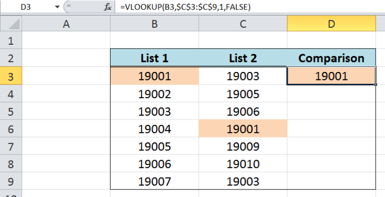 Figure 3. Excel VLOOKUP returning matched value in two columns
For the next value in column B, “19002”, the VLOOKUP function returns “#N/A” in cell D4 because “19002” is not found in column C.
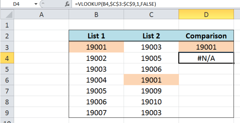 Figure 4. VLOOKUP returning #N/A for unmatched value
Below table shows the final results after comparing the two lists using VLOOKUP. The values 19001, 19003, 19005 and 19006 are present in the two lists.
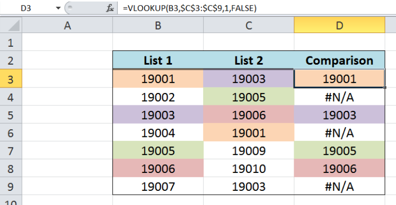 Figure 5. Using VLOOKUP to compare two columns in Excel
Compare two columns in Google sheets using VLOOKUP
In the same way, we can compare two columns in Google sheets using VLOOKUP by following the same procedure above. We insert the following formula into D3 and drag it down to D9.
=VLOOKUP(B3,$C$3:$C$9,1,FALSE)
The results of comparison in Excel and Google sheets is the same, as shown in the table below:
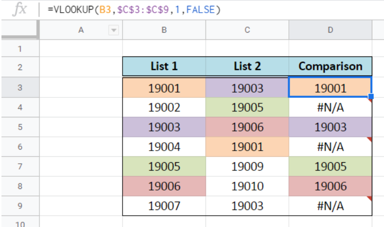 Figure 6. Using VLOOKUP to compare two columns in Google sheets
Compare two columns using Excel COUNTIF
While working with Excel or Google sheets and we want to count the number of times a value in one column exists in another column, we can use the function COUNTIF.
Syntax of COUNTIF Function
=COUNTIF(range,criteria)
- range – the data range that will be evaluated using the criteria
- criteria – the criteria or condition that determines which cells will be counted
In order to determine the number of times that a value in column B exists in column C, we follow these steps:
Step 1. Enter the formula in cell D3: =COUNTIF($C$3:$C$9,B3)
Step 2. Press ENTER
Step 3: Copy the formula in cell D3 to cells D4:D9 by clicking the “+” icon at the bottom-right corner of cell D3 and dragging it down
Our range is the set of values in column C, $C$3:$C$9. The criteria is B3, or the value in column B. The function returns the frequency of B3 in the range in column C. As a result, the value in cell D3 is “1”, because “19001” is found once in column C.
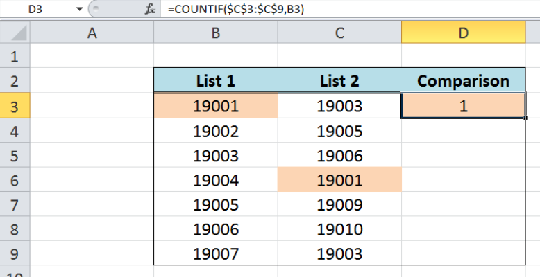 Figure 7. Excel COUNTIF returning the count for a matched value in two columns
As for B4, or “19002”, the COUNTIF function returns “0”, because “19002” is not found in column C.
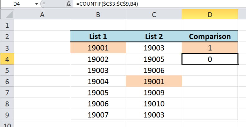 Figure 8. COUNTIF returning “0” for unmatched value
The value in D5 is “2” because “19003” is found twice in column C, specifically in C3 and C9.
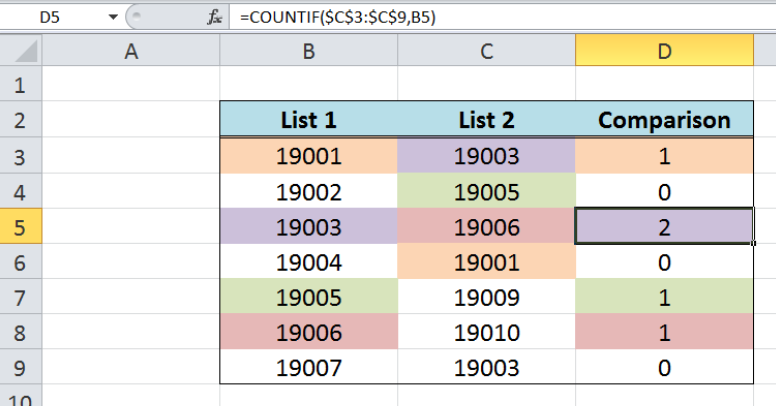 Figure 9. Using COUNTIF to compare two columns in Excel
Customize the result using IF and COUNTIF
We can customize the results when we compare two columns in Excel by combining the IF and COUNTIF functions. We follow the same procedure as in the previous example but we will be using this formula:
=IF(COUNTIF($C$3:$C$9,B3)>0,"Match found","Not found")
Instead of returning the count of matched values in the two lists, the formula returns “Match found” when the value in column B exists in column C, and returns “Not found” if otherwise.
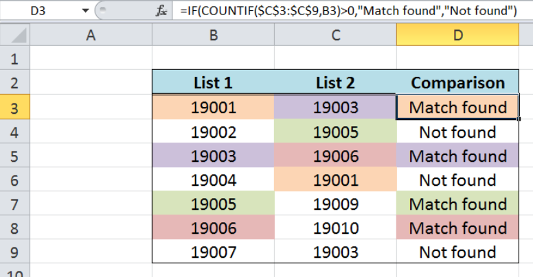 Figure 10. Using IF and COUNTIF to customize results
Compare two columns using MATCH
When we compare two columns in Excel, we might want to return the position of a value in a specified column, instead of the value itself. The MATCH function is the perfect solution for this, as it returns the position of a value in a specified range. Note, however, that it only considers the first match.
Syntax of the MATCH function
=MATCH(lookup_value, lookup_array, [match_type])
- lookup_value – a value which we want to find in the lookup_array
- lookup_array – the range of cells containing the value we want to match
- [match_type] – optional; the type of match; if omitted, the default value is 1; We use 0 to find an exact match
In order to determine if a value exists in two columns B and C and return its position instead of the value itself, we follow these steps:
Step 1. Enter the formula in cell D3: =MATCH(B3,$C$3:$C$9,0)
Step 2. Press ENTER
Step 3: Copy the formula in cell D3 to cells D4:D9 by clicking the “+” icon at the bottom-right corner of cell D3 and dragging it down
Our lookup_value is the value in column B, while our lookup_array is the set of values in column C, $C$3:$C$9. The match_type is “0” in order to find the exact match.
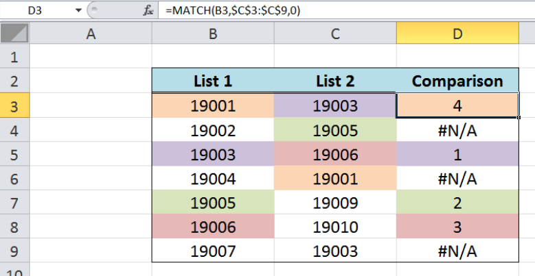 Figure 11. Using Excel MATCH to return positions of matched values in two columns
As a result, the value in cell D3 is “4”, because the value in column B “19001” is found in the fourth position (C6) in the lookup_array C3:C9. On the other hand, when a value is not found, the function returns “#N/A”, which is the case for D4, D6 and D9.
For “19003”, there are two matches in column C, specifically C3 and C9. However, MATCH function only considers the first match and disregards any other matches. In D5, the result is “1”, because the first match for “19003” is in the 1st position in the range C3:C9.
Compare two columns using INDEX and MATCH
A combination of INDEX and MATCH functions is used when we want to match two columns in our Google sheets or in Microsoft Excel. The MATCH function, as discussed above, returns the position of a value in a specified column while INDEX function returns the value of a cell in a range based on a column and row number.
Syntax of the INDEX function
=INDEX(array, row_num, column_num)
- array – a range of cells where we want to retrieve some data
- row_num – the row in the array from which we want to retrieve data
- column_num – the column in the array from which we want to retrieve data; if the array has only one column, column_num can be omitted
In order to compare the two columns B and C and return the matched value by using INDEX and MATCH, we follow these steps:
Step 1. Enter the formula in cell D3: =INDEX($C$3:$C$9,MATCH(B3,$C$3:$C$9,0))
Step 2. Press ENTER
Step 3: Copy the formula in cell D3 to cells D4:D9 by clicking the “+” icon at the bottom-right corner of cell D3 and dragging it down
Our array is the set of values in column C, $C$3:$C$9, and the row number is provided by the MATCH function.
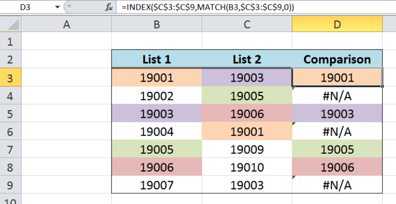 Figure 12. Using Excel MATCH and INDEX to return matched values in two columns
In the first example, our MATCH function looks up B3 or “19001” in the range C3:C9, and returns “4” which is the position of “19001” in the range C3:C9. The INDEX function then returns the fourth value in the array C3:C9, which is C6 or “19001”. The column number is ignored because we are considering only one column in our array, column C.
Finally, the value in cell D3 is “19001”. The combination of INDEX and MATCH when used to compare two columns yields the same results as when we are using VLOOKUP.
Compare two columns using Conditional Formatting
Conditional formatting is another built-in function in Excel or Google sheets that helps us compare two columns based on a set of rules.
Highlight duplicate values in two columns
Suppose we want to compare two columns in Excel and highlight the matches or duplicate values in B and C. We follow these steps:
Step 1. Select the cells we want to highlight, B3:C9.
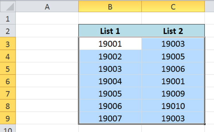 Figure 13. Selecting the cells to highlight matches in two columns
Step 2. Click the Home tab, Conditional Formatting Menu and select “Highlight Cells Rules”, then “Duplicate Values”. The Duplicate Values dialog box will pop up.
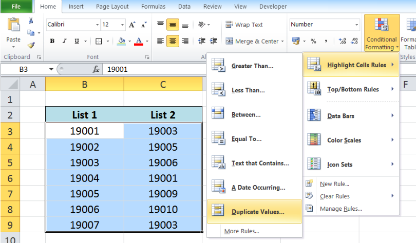 Figure 14. Creation of a new rule in Conditional Formatting
Step 3. In the Duplicate Values dialog box, select “Duplicate” and “Light Red Fill with Dark Red Text” in the drop-down lists
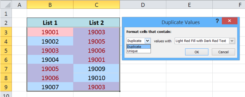 Figure 15. Formatting duplicate values in two columns
Step 4. Press OK to apply the formatting rule.
As a result, the duplicate values 19001, 19003, 19005 and 19006 in the two columns B and C are highlighted.
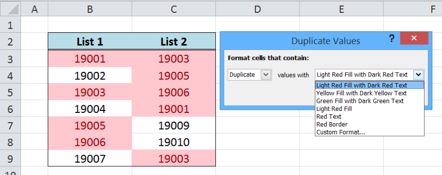 Figure 16. Output: Formatting rule reflected in duplicate values
Highlight unique values in two columns
We can also compare two columns in Excel and highlight the differences and use conditional formatting to highlight only the unique values. We follow the same procedure but this time, we choose “Unique” from the drop-down list and choose any format we want. In this case, we choose the formatting style “Yellow Fill with Dark Yellow Text”.
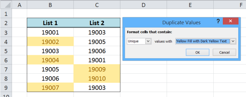 Figure 17. Output: Formatting rule reflected in unique values
As a result, the unique values 19002, 19004 and 19007 in the two columns B and C are highlighted.
Most of the time, the problem you will need to solve will be more complex than a simple application of a formula or function. If you want to save hours of research and frustration, try our live Excelchat service! Our Excel Experts are available 24/7 to answer any Excel question you may have. We guarantee a connection within 30 seconds and a customized solution within 20 minutes.
Are you still looking for help with the IF function? View our comprehensive round-up of IF function tutorials here.


Leave a Comment