

We can combine the use of Excel VLOOKUP and SUM functions to help us to quickly locate a specified criteria and also also sum up the presented values. We can look_up any specified criteria and then sum any other values related with the criteria values.
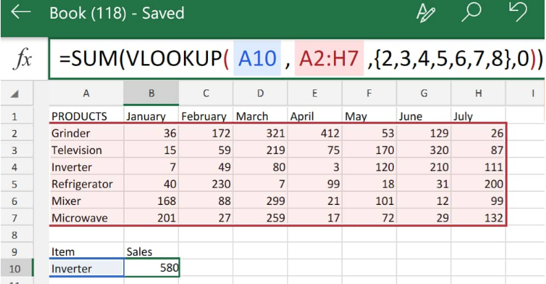 Figure 1. VLOOKUP SUM in Excel
SUM VLOOKUPS are essentially a combination of the Excel VLOOKUP with SUM functions in a single formula which we can then use to vlookup sum multiple matches in the columns or rows of our worksheet.
Generic Formula
=SUM(VLOOKUP(look_up value,look_up range,{column index},FALSE))
- Look_up Value = This is the specified value we are to search for and determine the sum of exact matches.
- Look_up Range = This is the cell range containing the data which is helpful to our search by using a specific criteria.
- Column Index = These are numbers used to calculate the total of the range of indexes that should be entered. We can enter all our column indexes or a few column indexes based on our requirements. These can be useful for identifying all of the columns included in our sum.
- Logical Value = This is an appropriate logical value. We can use either 0,1 or true,false values to select any matching values.
When we are working with numerical Excel data, quite often we are required to extract multiple associated values from a different work table and also sum these multiple number values inside several rows or columns. To accomplish this, we can combine SUM with VLOOKUP operations as demonstrated below:
How to SUM VLOOKUP in Excel
- We can start by collecting the available data inside our Excel sheet;
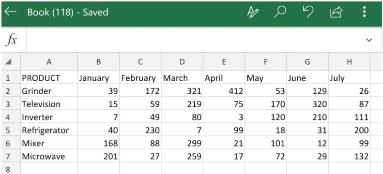 Figure 2. Data for SUM VLOOKUP in Excel
In the work table illustrated above, we have the amount of sales items made at a shop over a period of 7 months.
Our goal here is to look up an item in a row and use Excel SUM VLOOKUP to determine the total amount of that item sold. The generated VLOOKUP SUM rows formula we will enter into cell A10 of our work table is as follows;
=SUM(VLOOKUP(B10,A2:H7,{2,3,4,5,6,7,8},0))
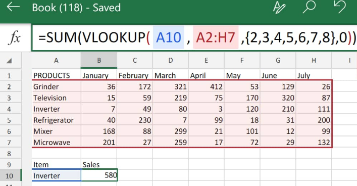 Figure 3. SUM VLOOKUP Function in Excel
Excel returned the VLOOKUP SUM of all matches to our specified criteria in cell A10 (inverter) as 580. Which represents the total sum of inverters that were sold from January to July.
Instant Connection to an Excel Expert
Most of the time, the problem you will need to solve will be more complex than a simple application of a formula or function. If you want to save hours of research and frustration, try our live Excelchat service! Our Excel Experts are available 24/7 to answer any Excel question you may have. We guarantee a connection within 30 seconds and a customized solution within 20 minutes.


Leave a Comment