

We can carry out a trend analysis in Excel when we want to know the percentage change of events over a period of two or more years. Trend analysis is so crucial if you want to know the underlying patterns in the past and current data movements. This will help you future behavior of what you are studying. It is thus necessary for learn how to calculate trend analysis in Excel. In this post, we shall look at a number of ways to calculate trend in Excel.
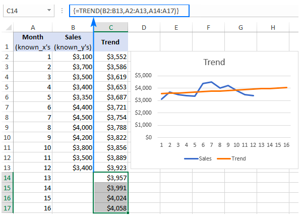 Figure 1: How to calculate trend in Excel
Calculating trend in Excel using Excel TREND function
We can utilize the Excel TREND formula to find a linear trend line that passes through a set of dependent valuables, Y and optionally through a set of independent variables, X.
Note that the TREND formula can help us extend the trend line into the future that be able to predict the Y-values for a set of new x-values.
=TREND (known_y’s, [known_x’s], [new_x’s], [const])
In the above Excel TREND formula, we have;
Known_y’s- represents a set of y-values that we already know. The known_y’s are required if the Excel trend function is to work correctly.
Known_x’s- represents sets of the independent x-values. Not mandatory.
How to use the TREND function to calculate trend analysis in Excel
When you have trending data in Excel, the Excel TREND function uses it to find the line that best fits that data using least squares method. If we have one range of x values, then the equation of the formula shall look as the one below;
Y= bx + a
In the event that we have multiple values of x, then the trend formula shall look as the one below;
Y= b1x1+b2x2+….+ bnxn+a
Where;
- y – is the dependent variable we are trying to calculate
- x – independent variable being used to find y
- a – is the intercept
- b – is the slope
When using the TREND function in Excel, one has to remember that it must be entered as an array formula. An array formula is entered by pressing Ctrl + Shift + Enter simultaneously. This is especially important when we want to have multiple y-values.


Leave a Comment