

Excel allows us to strip non-numeric characters from the string by using several Excel functions: TEXTJOIN, IFERROR, MID, ROW and INDIRECT. This step by step tutorial will assist all levels of Excel users in extracting the numeric characters from the text.
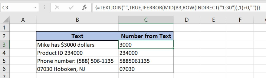 Figure 1. Remove non-numeric characters from the text
Syntax of the TEXTJOIN Formula
=TEXTJOIN(delimiter, ignore_empty, text1, [text2], ...)
The parameters of the TEXTJOIN function are:
- delimiter – a string that will be used as a separator between the text items
- ignore_empty – TRUE for ignoring empty cells
- text1, [text2] – text strings that will be joined
Syntax of the IFERROR Formula
=IFERROR(value, value_if_error)
The parameters of the IFERROR function are:
- value – a cell that is evaluated
- value_if_error – value to be inserted if an error exists in a cell
Syntax of the MID Formula
=MID(text, start_num, num_chars)
The parameters of the MID function are:
- text – a string from which we want to extract the characters
- start_num – position of the first character that we want to extract from the string
- num_chars – a number of characters that we want to extract from the first character
ROW and INDIRECT are helper functions in the MID formula array syntax and explanation for this formula part will be provided through the example.
Setting up Our Data for Stripping Non-numeric Characters
Our table consists of 2 columns: “Text” (column B) and “Number from Text” (column C). The idea is to strip non-numeric characters from the string and to place the numeric characters in column C.
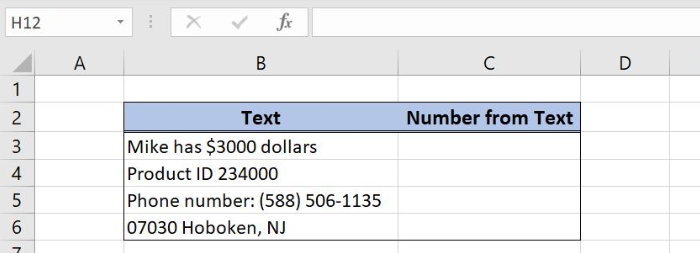 Figure 2. Table structure with cells containing text and numbers
Get numeric characters from the string
We want to extract only numeric characters from the string in column “Text”. This can be done with the combination of several functions: TEXTJOIN, IFERROR, MID, ROW and INDIRECT.
The formula looks like:
={TEXTJOIN("",TRUE,IFERROR(MID(B3,ROW(INDIRECT("1:30")),1)+0,""))}
A formula has to be an array function in order to work properly. To create an array function we have to click simultaneously ctr, shift, and enter on the formula.
To apply the formula we need to follow these steps:
- Select cell C3 and click on it
- Insert formula:
=TEXTJOIN("",TRUE,IFERROR(MID(B3,ROW(INDIRECT("1:30")),1)+0,"")) - Press ctrl, shift and enter simultaneously to create an array
- Drag the formula down to the other cells in the column by clicking and dragging the little “+” icon at the bottom-right of the cell.
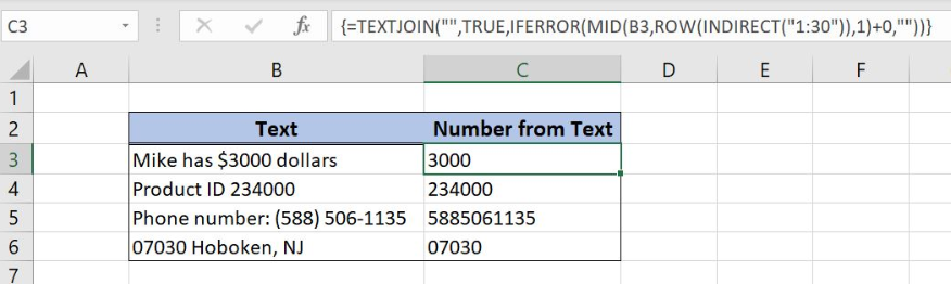 Figure 3. A formula for stripping non-numeric characters from the string
MID formula extracts each character of the string with the help of the formula part: ROW(INDIRECT(“1:30”)). Number ”1:30” in the INDIRECT formula means that MID function evaluates 30 characters of the string. We can enter a higher number if a string contains more characters.
MID function returns an array of 30 characters in a string:
{“M”;”i”;”k”;”e”;” “;”h”;”a”;”s”;” “;”$”;”3”;”0”;”0”;”0”;” “;”d”;”o”;”l”;”l”;”a”;”r”;”s”;””;””;””;””;””;””;””;””;}
We added 0 value after array because formula will display errors values whenever the character is the text:
{#VALUE!;#VALUE!;#VALUE!;#VALUE!;#VALUE!;#VALUE!;#VALUE!;#VALUE!;#VALUE!;#VALUE!;”3”;”0”;”0”;”0”;#VALUE!;#VALUE!;#VALUE!;#VALUE!;#VALUE!;#VALUE!;#VALUE!;#VALUE!;#VALUE!;#VALUE!;#VALUE!;#VALUE!;#VALUE!;#VALUE!;#VALUE!;#VALUE!}
IFERROR function replaces error values with an empty string:
{“”;“”;“”;“”;“”;“”;“”;“”;“”;“”;”3”;”0”;”0”;”0”;“”;“”;“”;“”;“”;“”;“”;“”;“”;“”;“”;“”;“”;“”;“”;“”}
Finally, TEXTJOIN function removes the empty strings and only numeric characters remain as a result: 3000.
Most of the time, the problem you will need to solve will be more complex than a simple application of a formula or function. If you want to save hours of research and frustration, try our live Excelchat service! Our Excel Experts are available 24/7 to answer any Excel question you may have. We guarantee a connection within 30 seconds and a customized solution within 20 minutes.


Leave a Comment