

Telephone numbers come in many forms, normally in combination with other characters like hyphens, periods and parentheses. While working with Excel, we are able to clean telephone numbers using the SUBSTITUTE function. This step by step tutorial will assist all levels of Excel users in cleaning and formatting telephone numbers.
 Figure 1. Final result: Clean and reformat telephone numbers
Final formula: =SUBSTITUTE(SUBSTITUTE(SUBSTITUTE(SUBSTITUTE(SUBSTITUTE(B5,"-",""),".",""),"(",""),")","")," ","")+0
Syntax of the SUBSTITUTE function
SUBSTITUTE function replaces a character or text in a text string
=SUBSTITUTE(text, old_text, new_text, [instance_num])
- text – the text string containing the character or text we want to replace or change
- old_text – any text that we want to replace with new_text
- new_text – the text we want to replace old_text with
- instance_num – Optional; Specifies which occurrence of old_text we want to replace; If omitted, every occurrence of old_text in text is replaced with new_text
Setting up Our Data
Our table has three columns: Telephone Number (column A), Clean Version (column B), Reformatted (column C). Note that the three telephone numbers listed have the same numbers but with different characters: dash “-”, period “.”, parentheses “()” and spaces.
In column B, we want to obtain the clean version of the telephone numbers, with only the numerical digits, without the other characters. In column C, we want to format the numbers according to our preference.
 Figure 2. Sample data to clean and reformat telephone numbers
Using the SUBSTITUTE function
Before we proceed to the final formula to clean telephone numbers, let us first learn how to use the SUBSTITUTE function.
Given below is the syntax for the SUBSTITUTE function:
=SUBSTITUTE(text, old_text, new_text, [instance_num])
For example, we want to substitute the dash “-” in cell B4 with an empty string. We enter the formula in cell C4: =(SUBSTITUTE(B4,”–“,“”))
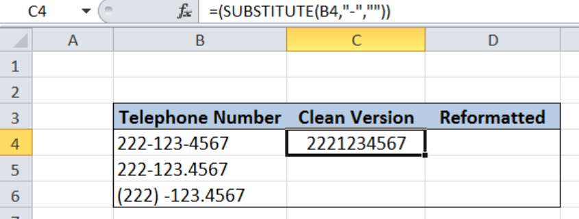 Figure 3. Entering the formula using SUBSTITUTE
The result in cell C4 is 2221234567, where the dashes are eliminated and only the numerical digits remain.
Clean telephone numbers
We want to obtain only the numerical digits of our telephone numbers and eliminate the other characters. The key here is to determine the characters that we want to eliminate and replace with the empty string. Looking at the telephone numbers, we want to substitute the dash “-”, the period “.”, the open and close parentheses “(“ and “)” and the space with an empty string “”.
We will be using one SUBSTITUTE function for every character that we want to replace with an empty string. In order to clean our telephone numbers, we follow these steps:
Step 1. Select cell C5
Step 2. Enter the formula: =SUBSTITUTE(SUBSTITUTE(SUBSTITUTE(SUBSTITUTE(SUBSTITUTE(B5,"-",""),".",""),"(",""),")","")," ","")+0
Step 3: Press ENTER
Step 4: Copy the formula in cell C5 to cell C6 by clicking the “+” icon at the bottom-right corner of cell C5 and dragging it down
 Figure 4. Using SUBSTITUTE to clean telephone numbers
Our formula is a combination of five SUBSTITUTE functions. The first SUBSTITUTE function becomes the text for the second SUBSTITUTE function, and so on. The additional “+0” at the end of the formula converts the telephone numbers into number format. This is especially helpful when we want to reformat our telephone numbers.
In cells C5 and C6, we have successfully cleaned the telephone numbers, leaving only the numerical digits 2221234567.
Reformat telephone numbers
First, let us copy the formulas of cells C4:C6 to cells D4:D6.
 Figure 5. Copying the formulas in column C to column D
In order to format the telephone numbers to our preference, let us follow these steps:
Step 1. Select cells D4:D6
Step 2. Press Ctrl + 1 to launch the Format Cells dialog box
Step 3: In the Format Cells dialog box, click Custom
Step 4. In the Type: box,enter the custom format: (###) ###-####
Step 5. Click OK.
 Figure 6. Entering the custom format
The format can be customized according to our preference. We can incorporate other characters, or change the color of the numbers.
For this example, our preferred format is (###) ###-####. As a result, we have now reformatted the telephone numbers in cells D4:D6.
 Figure 7. Output: Reformat telephone numbers
Most of the time, the problem you will need to solve will be more complex than a simple application of a formula or function. If you want to save hours of research and frustration, try our live Excelchat service! Our Excel Experts are available 24/7 to answer any Excel question you may have. We guarantee a connection within 30 seconds and a customized solution within 20 minutes.


Leave a Comment