

Excel allows a user to create a basic inventory formula example, by using the SUMIF function. This step by step tutorial will assist all levels of Excel users in creating a basic inventory formula example.
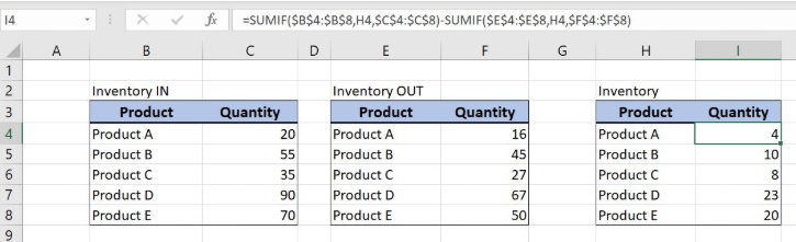 Figure 1. The result of the SUMIF function
Syntax of the SUMIF Formula
The generic formula for the SUMIF function is:
=SUMIF(range, criteria, [sum_range])
The parameters of the SUMIF function are:
- range – a range where we want to apply our criteria
- criteria – criteria which we want to apply to a range
- [sum_range] – a range where we want to sum. This is an optional parameter. If we omit it, the function will sum amounts from a range parameter.
Setting up Our Data for the SUMIF Function
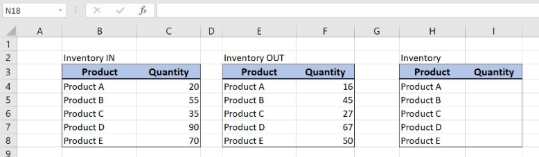 Figure 2. Data that we will use in the basic inventory formula example
We have 3 tables with two columns: “Product” and “Quantity”. The first table represents the quantity which came to the inventory, while the second represents the quantity which left the inventory. In the third table, we want to get the current inventory quantity by subtracting quantities from the first two tables. The result will be in column I.
Create a Basic Inventory Formula by the SUMIF Function
In our example, we want to subtract values in column F from values in column C, based on the products.
The formula looks like:
=SUMIF($B$4:$B$8, H4, $C$4:$C$8) - SUMIF($E$4:$E$8, H4, $F$4:$F$8)
For the first SUMIF, the parameter range is $B$4:$B$8 and the criteria is in the cell H4. The sum_range is $C$4:$C$8. For the second SUMIF, the parameter range is $E$4:$E$8 and the criteria is in the cell H4. The sum_range is $F$4:$F$8.
We have to fix range and sum_range parameters, as they are not changing when the formula is copied down the cells.
To apply the SUMIF function, we need to follow these steps:
- Select cell I4 and click on it
- Insert the formula:
=SUMIF($B$4:$B$8,H4,$C$4:$C$8)-SUMIF($E$4:$E$8,H4,$F$4:$F$8) - Press enter
- Drag the formula down to the other cells in the column by clicking and dragging the little “+” icon at the bottom-right of the cell.
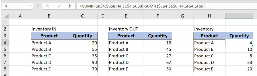 Figure 3. Counting the cells that begins with a certain text
As you can see in Figure 3, the quantity for Product A in the first table is 20 and in the second table is 16. When we subtract these two values, we get quantity 4 in the cell I4.
Most of the time, the problem you will need to solve will be more complex than a simple application of a formula or function. If you want to save hours of research and frustration, try our live Excelchat service! Our Excel Experts are available 24/7 to answer any Excel question you may have. We guarantee a connection within 30 seconds and a customized solution within 20 minutes.


Leave a Comment