

The SUMIF function in Excel is designed for only one criterion or condition. When we need to sum values based on multiple criteria, we can add two or more SUMIF functions, or we use a combination of SUM and SUMIF functions. Here’s how.
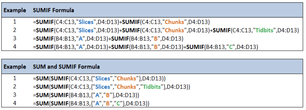
Figure 1. SUMIF combined with multiple criteria
Setting up the Data
Here we have an inventory of stocks for five different products stored in four warehouses.
We want to determine the following:
- Total stocks for Slices and Chunks
- Total stocks for Slices, Chunks and Tidbits
- Total stocks in Warehouse A and B
- Total stocks in Warehouse A, B and C
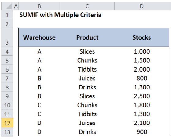 Figure 2. Sample table for SUMIF combined with multiple criteria
SUMIF function in Excel
SUMIF is a function that sums the values in a specified range, based on one criterion.
Syntax
=SUMIF(range,criteria, [sum_range])
Where
- Range: the data range that will be evaluated using the criteria
- Criteria: the criteria or condition that determines which cells will be added
- Sum_range: the cells that will be added; if left blank, “sum_range” = “range” which means that the range of data that will be added is the same range of data evaluated
Example of SUMIF with one criterion:
Determine the total stocks for Slices.
In cell G4, enter the formula: =SUMIF(C4:C13,”Slices”,D4:D13)
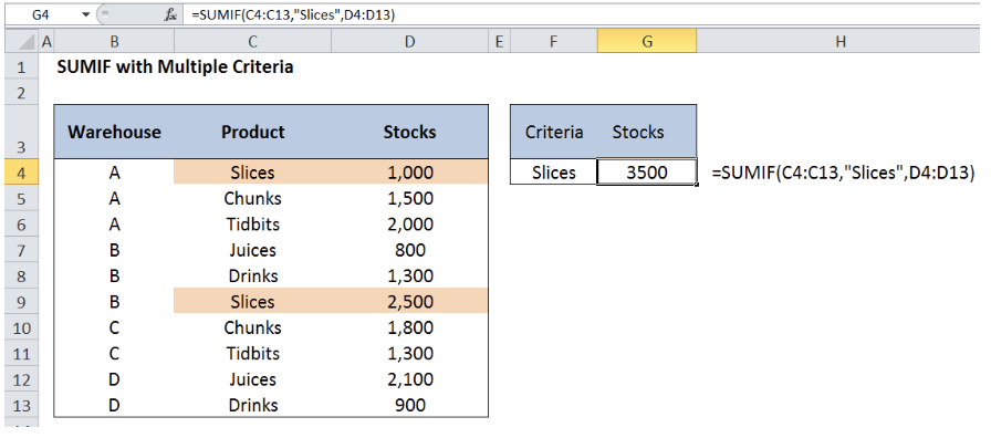 Figure 3. Entering the formula for SUMIF with one criterion
The total stocks for Slices is 3,500: 1,000 in Warehouse A and 2,500 in Warehouse B.
SUMIF Combined with Multiple Criteria
For multiple OR criteria in the same field, we use several SUMIF functions, one for each category.
Syntax
=[SUMIF] + [SUMIF]+...
=SUMIF(range1, criteria1, [sum_range1]) + SUMIF(range2, criteria2, [sum_range2])+...
This formula works like an OR logical formula, which sums values for every criteria that is satisfied.
We want to determine the following:
- Total stocks for Slices and Chunks
- Total stocks for Slices, Chunks and Tidbits
- Total stocks in Warehouse A and B
- Total stocks in Warehouse A, B and C
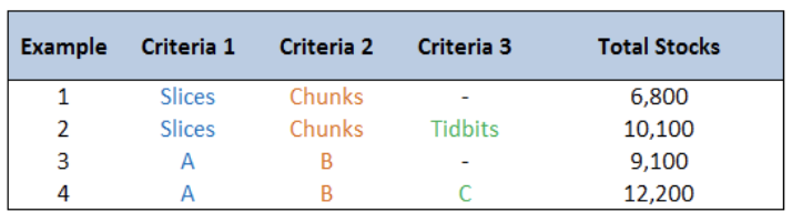 Figure 4. Examples for SUMIF combined with multiple criteria
Example 1: Total stocks for Slices and Chunks
In cell J4, enter the formula:
=SUMIF(C4:C13,"Slices",D4:D13)+SUMIF(C4:C13,"Chunks",D4:D13)
where
- SUMIF(C4:C13,”Slices“,D4:D13) : sum of stocks for Slices
- SUMIF(C4:C13,”Chunks“,D4:D13): sum of stocks for Chunks
The total stocks for Slices and Chunks is 6,800.
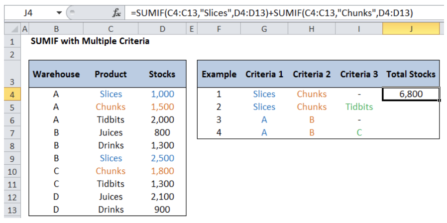 Figure 5. Entering the formula for SUMIF with multiple criteria
Examples 2 to 4:
For the other examples, enter the formula as shown below:
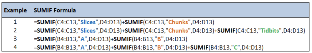 Figure 6. Formula for SUMIF combined with Multiple Criteria
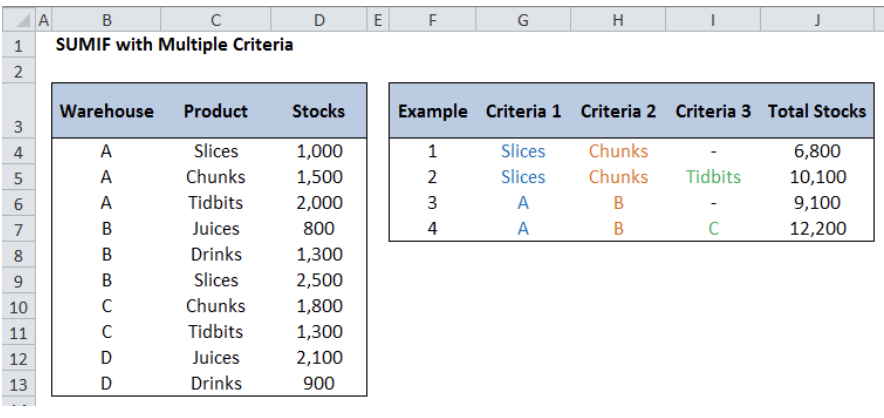 Figure 7. Output for SUMIF combined with Multiple Criteria
We must not get caught up with how many conditions need to be satisfied. When using SUMIF combined with multiple criteria, we must remember that for each criterion, there must also be one SUMIF function. This way, we will never be intimidated with any related problem in the future.
Alternative Formula using SUM and SUMIF
When there are more and more criteria to satisfy, the summation of SUMIF formula will become very long and tedious. Here is an alternative formula using SUM and SUMIF functions.
Syntax
=SUM(SUMIF(range,{criteria1,criteria2,criteria3},sum_range))
Let’s take the first example where we sum the stocks for “Slices” and “Chunks”.
OLD Formula: “=SUMIF(C4:C13,"Slices",D4:D13)+SUMIF(C4:C13,"Chunks",D4:D13)”
This time, the formula is shorter and simpler:
New Formula: “=SUM(SUMIF(C4:C13,{"Slices","Chunks"},D4:D13))”
Refer to below table and see the difference of the two methods:
Figure 8. Comparison of two methods in using SUMIF combined with multiple criteria
Most of the time, the problem you will need to solve will be more complex than a simple application of a formula or function. If you want to save hours of research and frustration, try our live Excelchat service! Our Excel Experts are available 24/7 to answer any Excel question you may have. We guarantee a connection within 30 seconds and a customized solution within 20 minutes.


Leave a Comment